Introduction

Towards the end of their evolution, stars with masses greater than about $8 M_\odot$ explode, producing one of the most energetic observable events in our Galaxy and external galaxies. The generally accepted sequence of events leading to this outcome is as follows. A star is said to have formed when a self-gravitating cloud of gas (mostly hydrogen) collapses under its own gravity to densities and temperatures at which, hydrogen burning begins. Under the action of gravity, the centre gets denser and hotter resulting into a well defined series of nuclear reactions. These reactions, starting from hydrogen burning and going all the way to the formation of iron, start at the centre and feed on the products of earlier reactions, which continue to occur further out. With time, a series of concentric shells are formed around the core, consisting of various elements produced in the these reactions. This model is usually referred to as the ``onion-skin model'' with a core of iron surrounded by shells of lighter elements with the outer most shell consisting of hydrogen (and possibly some He, Ne, O, N and C). Simulations show that, depending upon the initial masses, some stars complete the full sequence of nuclear reactions while for others this sequence is interrupted (Woosley & Weaver1986; Trimble1982, and references therein). Single stars with initial masses greater than about $8 {M_\odot}$, explode producing Type II supernovae (SNe) which are characterized by the presence of hydrogen lines in their spectra and are usually found in the spiral arms for spiral galaxies. Type I SNe on the other hand are produced due to a white dwarf reaching the critical mass due to accretion from a companion star in a binary system. These SNe are devoid of hydrogen lines in their spectra and occur in all types of galaxies. The star is completely disrupted in the case of Type I SNe and no compact core remains (Woosley & Weaver1986). The central part of the iron core in Type II SNe, however, is compressed to nuclear densities and is left behind as a spinning degenerate neutron star, which is, in some cases, detected as a pulsar. After the core collapse, the rest of the material which is still in-falling, rebounds (since the neutron core cannot be further compressed) creating a powerful shock wave which ploughs though the the outer layers of the star and finally emerges out of the circumstellar material. The core collapse releases $10^{53}$ erg of gravitational energy in the form of neutrinos which, along with the blast wave, couple with the outer layers and eject them at high speeds. The explosion in both types of SNe releases $\sim 10^{51}$ erg of kinetic energy, which produces a shock wave travelling outwards. The cores of massive stars with initial masses in the range of $18-30 {M_\odot}$ can also first explode as SNe and then collapse into low mass black holes (Brown & Bethe1994). In such an event, a heavy star collapses into a black hole without returning matter to the galaxy. The empirical value of $\Delta Y/\Delta Z$ (the relative helium to metal enrichment) implies a maximum mass of the star, after which the nucleosynthesis must cut off (i.e., stars more massive than this limit cannot contribute higher metals to the galaxy). This maximum mass limit derived from the value of $\Delta Y/\Delta Z$ and that derived from the computation by Brown & Bethe (1994) are in good agreement.

Figure 1.1: Initial radio light curves at 6 and 20 cm of a Type II-L SNe SN1980k taken from Weiler et al. (1986). Such light curves are thought to be typical of the class. The data points marked by crosses and filled circles are measured flux densities while the solid curves are the best fit theoretical curves. Emission at 6 cm starts and peaks earlier than at 20 cm. The emission initially increases rapidly, reaches a maximum value and then monotonically decays at both the frequencies.

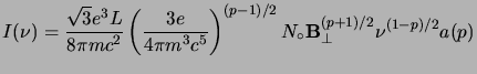
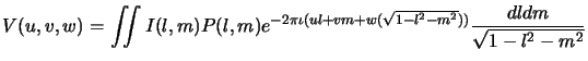
The interaction of the above shock wave with the in-falling circumstellar material produces the initial radiation, which announces the onset of the explosive event to observers on Earth. The shape of the initial optical light curve and the spectra at the peak of optical emission can be used to differentiate between the Type I and Type II SNe (Weiler & Sramek1988). Type-I SNe are characterized by the absence of hydrogen lines in their peak optical spectra while Type-II exhibit hydrogen lines in their spectra. Based on further finer details of the light curve, SNe are further sub-divided into Type Ia, Ib, II-L (linear) and II-P (plateau). However, initial radio emission has been detected from Type-Ia SNe. The optical light curve of Type II-L decreases monotonically in intensity after reaching a peak value while that of Type II-P, on the other hand goes through a flat plateau before starting to decay further. The peak absolute blue magnitude of Type Ia SNe has been found to be remarkably constant for different events; these can hence be used as ideal standard candles in the universe. Hubble constant can therefore be derived from the observations of extragalactic Type Ia SNe light curves. It is this property of Type Ia SNe which is responsible for the currently thriving industry of Supernova Cosmology (Branch1998, and references therein).

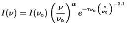
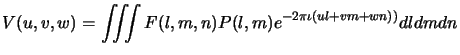
Typically, radio emission is first detected at higher frequencies, and later, at successively lower frequencies due to changes in the optical depth for external free-free absorption (Weiler et al.1986). A typical example of radio light curve for a Type II-L SN is shown in Fig. 1.1. The shape and spectral behavior of this initial radio light curve is thought to be typical of the class. Radio emission is detected significantly after the optical light is detected. The spectral index $\alpha$ ( $S_\nu\propto\nu^\alpha$) evolves from a value of $\sim1$ to a relatively constant value of $\sim-0.7$ when the emitting region becomes optically thin for radio photons (Fig. 1.2). Observations of SN1983N, a Type Ib SN, on the other hand, exhibited a far more rapid rise as well as decay in the flux density compared to that of Type II-L SN. This difference in the radio light curves of the two types have been interpreted as being due to significant differences between the environments of Type Ib and II-L SNe.

After the blast wave crosses the denser circumstellar envelope into the more tenuous interstellar medium (ISM), this initial radio emission ultimately dies down, over time scales of several weeks for Type I SNe to many years for Type II SNe. The evolution of the blast wave as it ploughs though the ISM can be roughly described in four distinct stages (Reynolds & Chevalier1984). This interaction of the blast wave with the ISM, at much later times, produces sources of synchrotron emission in the sky, called Supernova Remnants (SNRs). SNRs are visible at radio bands (and at optical and X-ray bands in regions where the obscuration by the Galactic plane is relatively low) for up to $\sim 10^4-10^6$ years after the initial explosion. This dissertation is concerned with the observations of such Galactic SNRs at low radio frequencies.

Figure 1.2: Spectral index evolution between 6 and 20 cm for a Type II-L SNe SN1979c taken from Weiler et al. (1986). The solid curve corresponds the best fit curve derived from the flux densities measured at these wavelengths.

Synchrotron Radiation

A relativistic electron moving at a velocity v in the presence of magnetic field of strength B, moves in a helical path around the field line, and consequently emits synchrotron radiation (Ginzburg & Syrovatskii1969; Moffet1975, and references therein). A brief description of the synchrotron emission mechanism and the results which follow is taken from Salter & Brown (1988). If the angle between the v and B vectors (the pitch angle) is $\theta$ and the total energy of the electron is $E=\gamma mc^2$ where $\gamma = 1/(1-v^2/c^2)^{1/2}$ is the Lorentz factor, the frequency of gyration around the field lines is given by

$$\nu_g = \frac{e{\bf B}_\perp}{2 \pi \gamma m c} = \frac{\nu_\circ}{\gamma}$$ (4.1)

where ${\bf B}_\perp = {\bf B}\sin \theta$ is the component of the magnetic field perpendicular to the electron path and $\nu_\circ$ is the non-relativistic electron gyro-frequency. Due to relativistic effects, the radiation will be emitted in a narrow cone of half-angle of the order of $1/\gamma$. In general, a detector will detect pulses of radiation from such a system every time the the cone of emission crosses the detector's line of sight and the pulse shape will be defined by a cut across the cone of emission. The frequency of the pulses as seen by the detector will be the Doppler shifted gyration frequency given by

$$\nu^\prime_g \sim \frac{\nu_g}{\sin^2 \theta}$$ (4.2)

while the pulse width is

$$\Delta t \sim \frac{1}{2 \pi \nu_g \gamma^3}$$ (4.3)

Since the width of the individual pulses will be narrow (at least for large values of $\gamma$), most of the emitted energy will be in harmonics of the fundamental frequency given by $(2\pi\Delta t)^{-1}\sim\nu_g\gamma^3$. For ultra-relativistic electron, these harmonics will be closely spaced and the resulting spectrum is essentially a continuum. The critical frequency at which the emission is maximum is given by

$$\nu_c = \frac{3}{2} \gamma^2 \nu_\circ = 16.08 \times 10^6 {\bf B}_\perp E^2 \mathrm{MHz}$$ (4.4)

where $E$ is the electron energy in GeV and ${\bf B}_\perp$ in gauss. The rate of loss of energy by the electron due to synchrotron radiation is given by

$$\frac{dE}{dt} = -119.7 {\bf B}^2_\perp E^2 \mathrm{GeV/yr}$$ (4.5)

This basic equation says that the most energetic electrons will lose energy at the fastest rate. With time, a high energy electron will lose energy and radiate for longer as a lower energy electron. For an ensemble of electrons with some initial energy distribution, with time time, more electrons will pile up at the lower energy end of the energy spectrum. This produces observable changes in the properties of the emission with time. This effect goes by the name of ``ageing'' in the literature.

For a homogeneous and isotropic ensemble of electrons with energy density distribution $N(E)dE$, the total intensity will be given by

$$I(\nu) = \int\limits_0^\infty N(E) P(\nu) dE$$ (4.6)

where $P(\nu)$ is the spectrum of the electron with energy in the range between $E$ and $E+dE$. For a power law energy spectrum given by $N(E)dE=N_\circ E^{-p}dE$ in a limited range $E_1 < E < E_2$, $I(\nu)$ is given by

$$I(\nu)=\frac{\sqrt{3}e^3L}{8\pi m c^2}\left(\frac{3e}{4 \pi m^3 c^5}\right)^{(p-1)/2} N_\circ {\bf B}^{(p+1)/2}_\perp \nu^{(1-p)/2} a(p)$$ (4.7)

where $a(p)$ is a slowly varying function of $p$ and $L$ is the spatial extent of the region with uniform magnetic field B. Clearly, for a power law distribution of initial energies, $I(\nu) \propto \nu^\alpha$ where $\alpha$ is the spectral index and is related to $p$ as $\alpha = (1-p)/2$. $p$ is usually greater than unity; a negative spectral index is thus observational evidence for synchrotron emission.

Emission from a single electron will clearly be elliptically polarized with the electric field vector perpendicular to the projected magnetic field vector. However, for an ensemble of electrons with a random distribution of pitch angles, the observed radiation will be partially linearly polarized with the degree of polarization in a uniform magnetic field given by

$$\Pi = \frac{p+1}{p+7/3}$$ (4.8)

Linear polarization and a negative spectral index are the two defining characteristics used to identify sources of synchrotron emission, although either is usually sufficient to identify the emission mechanism. Radiation can however be depolarized due to a variety of reasons ranging from random orientations of the magnetic field vectors within the resolution element of the telescope or thermal material along the line of sight to Faraday rotation in the Earth's ionosphere. Depolarization scales as $\lambda^2$ and consequently measurement of polarization at low frequencies is usually difficult. Hence, while detection of linearly polarized emission is a strong proof of synchrotron emission, a lack of it cannot rule it out. A negative spectral index is therefore frequently used as a signature of synchrotron radiation.

Galactic Supernova Remnants

A large number of SNRs are radio sources with only less than 30% visible in optical and X-ray bands. The lack of optical and X-ray radiation is primarily due to obscuration by the Galactic disk. Out of the 225 Galactic SNRs listed in the catalogue of Galactic SNRs (Green2000), about 80% are of shell-type morphology (see Section 1.2.4) with a median size of $\sim30$ arcmin. The emission is polarized (fractional polarization at $5-10\%$ level for the shell-type SNRs and much higher for filled centre SNRs) with a negative spectral index and is therefore believed to be synchrotron radiation. These gross observed radio properties of the radio emission from SNRs can be understood by modeling the shock wave as a spherical supersonic piston propagating in a uniform medium (the ISM) sweeping up the ISM mass as it moves. Its evolution is described as four distinct stages (Reynolds1988, and references therein):

• Free expansion phase

  In this stage of the evolution, the ejected mass $M_\circ$ is much more than the mass swept-up by the shock front, i.e. $M_\circ \gg 4\pi R_s^3\rho_1/3$ where $R_s$ is the shock radius and $\rho_1$ the pre-shock density. The influence of the ISM on the dynamics of the ejecta in this stage is negligible and the initial properties of the explosion dominate the evolution. Consequently the blast wave freely expands into the medium.

• Sedov phase

  With time, the shock front sweeps up the ISM material and enters this phase when the swept-up ISM mass is comparable to that of the ejected mass. The shock is still strong and the pressure due to the swept-up mass is negligible. The expansion is essentially adiabatic (which is the other name this phase goes by) and the dynamical evolution is given by Sedov (1959) solution for the dynamics of a point explosion in a uniform medium. For a gas with the ratio of specific heats of 5/3, the shock radius and velocity ($v_s$) are given by

  $$R_s = 1.17\left(\frac{E_\circ}{\rho_1}\right)^{1/5} t^{2/5}$$ (4.9)

  
  

  $$v_s = 0.4R_s/t$$ (4.10)

  
  
  where $E_\circ$ is the supernova energy. The ejecta begin to decelerate in this phase and a reverse shock develops which propagates into the ejecta, thus thermalizing it. The reverse shock propagating into the circumstellar material is thought to be responsible for the observed X-ray emission.

• Radiative phase

  Once the age of the remnant becomes comparable to the radiative cooling time scales near the shock, the blast wave enters the radiative phase. The deceleration becomes rapid and the shock compression becomes large. By this time, the dynamics and the resulting observed morphologies are significantly affected by the structure of the ISM, particularly the inhomogeneity of the ISM.

  The time at which this phase begins and the shock velocity at this time is given by

  $$t = 3.5\times 10^4\left(\frac{E_\circ}{10^{51} \mathrm{erg}}\right) n_1^{-9/17} \mathrm{yr}$$ (4.11)

  
  

  $$v = 230 n_1^{2/17}\left(\frac{E_\circ}{10^{51} \mathrm{erg}}\right)^{1/17} \mathrm{km s}^{-1}$$ (4.12)

  
  
  where $n_1$ is the pre-shock number density.

• Dissipative phase

  Once the expansion velocity of the shock decreases below the local sound speed, it dissipates and merges with the ISM on time scales of $10^5-10^6$ years.

This simple model of a shock wave propagating in a uniform medium, however, ignores a number of other effects such as dynamical effects of the magnetic field, pressure forces in the radiative phase and inhomogeneities in the ISM (Woltjer1972). Hydrodynamic calculations show that SNe produce ejecta with a uniform density towards the outer parts while the inner parts (close to the star) have a steep density profile (like $\rho\propto r^{-7}$). A reasonable density profile for Type I SNe has a constant density ejecta for the inner four-sevenths of the mass, and the outer three-sevenths obeying $\rho\propto r^{-7}$. Numerical simulations for Type I SNe with such a density profile modified the evolution of the shock radius to $R_s \propto t^{4/7}$ when the Sedov phase is reached, which is closer to the observed value of the exponent (e.g. for Tycho and SN 1006).

Nonthermal Emission from SNRs

As mentioned earlier, radio emission from SNRs is believed to be synchrotron radiation which requires understanding of the origin of the relativistic electrons and magnetic field. Broadly, the central pulsar is thought to be the source of both these quantities for Crab-like SNRs (see Section 1.2.4), while, for shell-type SNRs, both come from the ambient ISM. The inferred magnetic fields in SNRs, measured from the rotation measure measurements of background radio sources, X-ray observations and Zeeman splitting of OH maser lines (Brogan et al.2000), is however $\sim 2-3$ order of magnitude higher than the ambient magnetic field, requiring magnetic field amplification mechanisms as well. Although it is easy to imagine amplification of the frozen-in magnetic field in the SNR shells, the observed brightness of young shell-type SNRs is often more than can be explained by magnetic field amplification due to compression by the shock alone (although, magnetic field strengths measured for a few SNRs using the Zeeman splitting of OH (1720 MHz) lines are consistent with the hypothesis that ambient molecular cloud magnetic fields are compressed via the SNR shock to the observed values (Brogan et al.2000)). The observationally deduced magnetic field for Cas A is far too high to be explained by magnetic field amplification by compression by a factor 4 compression. Similarly, the deduced magnetic field for the shell-type Kepler's SNR (Matsui et al.1984) is too high to be produced by the amplification of the ambient field in the shock front. It is therefore believed that for shell-type SNRs, a combination of particle acceleration in the shock front (Bell1978a; Bell1978b) and magnetic field amplification as well as particle acceleration behind the shock (Cowsik & Sarkar1984; Gull1973) are responsible for the observed radio brightness. On the other hand, the observed properties and the evolution of Crab-type SNRs are believed to be dominated by rotational energy loss from the central pulsar (Reynolds & Chevalier1984).

Two classes of electron acceleration mechanisms have been used: turbulent acceleration at the unstable contact discontinuity and acceleration in the shock front itself. The first mechanism uses ``second-order Fermi acceleration'' and explains the morphology and emission from SNRs like Cas A. The latter mechanism uses the more efficient ``first-order Fermi acceleration''. This has the added advantage that the inferred electron energy spectra is naturally a power law and explains the morphology and the spectra of typical shell-type SNRs (Reynolds & Ellison1992). Mechanisms for magnetic field amplification are however far less well understood. Magnetic fields measured in a few SNRs are much too high to be explained by compression alone. Observed magnetic fields which are predominantly radial in young SNRs (Dickel & Milne1976) also argue against the amplified field being the swept-up ambient field. Magnetic field amplification in the Rayleigh-Taylor instability due to the deceleration of the ejecta (Jun et al.1996; Jun & Norman1996b; Jun & Norman1996a), is an attractive model, especially for clumpy ejecta and/or circulstellar medium in the sense that it can explain the mostly radial orientation of the magnetic field in the SNR shells. Their simulation also shows that such magnetic field amplification is dependent on the orientation of the field and can produce morphologies similar to those of ``barrel-shaped'' SNRs.

Continuum Radio Spectra

Although the details of the particle acceleration and magnetic field amplification mechanism are still not well understood, it is clear from the observed data that the radio emission from SNRs is synchrotron radiation. Radio emission from SNRs above $\sim 100$ MHz has a non-thermal spectrum (Equation 1.7) and significant linear polarization ($5-10$% for shell-type SNRs and up to 30% for filled centre SNRs). Both these gross properties are considered to be defining properties of synchrotron emission. Integrated continuum radio spectra are therefore the primary signatures used to identify SNRs. As is also obvious, SNRs also produce sources of extended emission. Radio SNRs are classified into roughly four categories (see Section 1.2.4) based on the radio morphology. Radio morphology also provides information about the SNR type, its interaction with the ambient ISM as well as with the ambient magnetic field (Dickel & Milne1976). Candidate SNRs are therefore often identified from single frequency observations based on the morphological evidence. However, H II regions in the Galaxy also exhibit extended radio emission easily detected at higher frequencies and, in some cases even exhibit morphologies similar to those of SNRs. Identifications of SNRs based on a single high frequency observation are therefore unreliable; observations at at least two frequencies are therefore usually required for proper identification of extended radio sources, to get a handle on the spectral index. Non-detection of thermal infrared emission, and where possible, lack of radio recombination lines (RRLs) are also used as supporting evidences to distinguish synchrotron sources from sources of thermal emission. However, RRL observations in the Galaxy are usually at coarse resolution and have a patchy coverage of the Galactic plane. High frequency observations in the Galactic plane also suffer from contaminating thermal emission (see Section 1.2.3), which has a relatively flat spectrum above $\sim1$ GHz. Below this frequency, typical thermal emission strongly turns over due to free-free absorption. Synchrotron emission on the other hand, has a negative spectral index for a large range of frequencies. As a result, the emission from SNRs is usually stronger at lower frequencies while the thermal emission is severely diminished. For these reasons, high resolution observations at low frequencies where the non-thermal emission is stronger than the thermal emission can identify SNRs unambiguously and also measure spatially resolved brightness variations. The latter provide crucial information about the interaction of the blast wave with the ISM as well about particle acceleration/magnetic field amplification.

The spectral index depends on the kinetic energy input mechanism (e.g. turbulence in the shells of shell-type SNRs and the central pulsar in Crab-type SNRs), localized particle acceleration mechanisms (e.g. interaction of the shock front with higher density ISM) and the properties of the intervening ISM (e.g. differential free-free absorption across SNRs). About 80% of the known Galactic SNRs are of shell-type (Green2000) and exhibit a broad range of spectral indices ( $-0.2 < \alpha < -0.8$) with a mean value of $\sim -0.5$. This implies a mean electron energy spectrum $\propto E^{-2}$, close to what is expected from theoretical models for acceleration in strong shocks. Implied electron energy spectra corresponding to the lower range of $\alpha$ are explained by attributing them to weaker shocks while those corresponding to the higher range require the inclusion of non-linear effects. Data also suggests a trend in the spectral index with the remnant age (i.e. with diameter). Smaller diameter SNRs, considered to be younger, have $\alpha < -0.5$ while older, larger diameter SNRs have flatter spectra. However it must also be kept in mind that the measured diameter is subject to (often large) errors in the distance estimate. Even if the distance is well known, the diameter of the SNR can be strongly influenced by the properties of the progenitor star and the local ISM and the inferred age may be quite different from the true age. Spectral indices for most SNRs have been obtained from measurements carried out with a variety of telescopes and techniques, resulting into uncertainties in flux density scales. As a result, the spectral indices are seldom known to accuracies better than $\sim 0.1$.

Measurements of spatial and/or temporal variations in the radio spectra of SNRs are probably the best way to study the nature of electron acceleration mechanisms. Spatial spectral variations provide information about the local dynamics and require spatially resolved observations at at least at two frequencies. High resolution observations are usually done using interferometric telescopes. However, the set of the spatial frequencies measured by such instruments with fixed physical separation between the antennas are a function of the observing frequency. As a result the spatial frequencies sampled at two different frequencies are in general different and dividing the two images at different frequencies to obtain spectral index maps produces artifacts. In telescopes like the Very Large Array (VLA) this problem is solved by scaling the array in proportion to the observing frequency, but for most other interferometric telescopes, this remains a problem. Observations with interferometric telescopes also suffer from missing larger scale emission which in turn result into differences in flux density base-level. Similarly, single dish observations also suffer from base-level problems due to very large scale background emission within the field of view of the telescope. To minimize the errors in the measurement of spectral index due to these effects, Anderson & Rudnick (1993) used the so called ``T-T plot'' to measure the local gradient in the maps at two frequencies. This method is insensitive to large scale base-level variations in the two maps and gives a more reliable spatially resolved spectral index measurement. They find a spatial variation from $-0.7$ to $-0.4$ across a few, hopefully representative, SNRs. More recently Katz-Stone et al. (2000a) used the method of spectral tomography to measure spectral variations within Tycho's SNR. They identified a number of filaments with spectral index different from that of the smoother background. The filaments in the outer rim show a trend such that brighter filaments have a flatter spectral index which could be due to the interaction of the blast wave with a inhomogeneous ambient medium or due to inhomogeneities in the magnetic field.

Absorption by the low density ionized medium

Figure 1.3: Plot showing a typical continuum spectra for Galactic SNRs. The spectral index at frequencies $>100$ MHz is clearly non-thermal. Below this frequency, the flux density decreases due to free-free absorption in the intervening low density ISM.

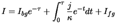
In their classic papers on the measurement of low-frequency continuum spectra of Galactic supernova remnants, Dulk & Slee (1975) reported spectral turnovers in several SNRs in the galactic plane at low frequencies. Such a turnover in the spectra of SNRs has since been confirmed by more extensive measurements at $\sim 31$ MHz (Kassim1989). The spectral index above $\sim 100$ MHz is negative and is typical of most SNRs (Fig.1.3^4.1). The spectra however turns-over below this frequency due to absorption by low density ionized gas in the intervening ISM (Kassim1989). The observed flux density at a frequency $\nu$ in the presence of absorbing foreground medium of free-free optical depth $\tau_{\nu_\circ}$ at a reference frequency $\nu_\circ$ can be written as

$$I(\nu) = I(\nu_\circ)\left(\frac{\nu}{\nu_\circ}\right)^\alpha e^{-\tau_{\nu_\circ} \left(\frac{\nu}{\nu_\circ}\right)^{-2.1}}$$ (4.13)

where $I(\nu)$ is in Jansky and the frequency $\nu$ is in MHz. $\tau_{\nu_\circ}$ is related to the emission measure EM(cm$^{-6}$ pc$^{-1}$), and the electron temperature $T_e$(K) (Dulk & Slee1975) by

$$\tau_\nu=1.643\times10^5 a\left(T_e,\nu\right)\left(\nu^{-2.1}\right)\left(EM T_e^{-1.35}\right)$$ (4.14)

where $a(T_e,\nu)$ is the Gaunt factor, $\sim1$ for the relevant range of $T_e$ and $\nu$. The emission measure EM is defined as

$$EM=\int_L n_e^2 dl$$ (4.15)

where $n_e$ is the thermal electron density in cm$^{-3}$ and the L is the path length to the source in parsec. With an estimate of the distance to an SNR and assuming that the spectral index is same at the range of frequencies under consideration, these equations can be used to estimate the properties of the absorbing gas, namely $\tau_\nu$ and $n_e$. The absence of a low frequency turn over towards distant SNRs places severe constraints on the thermal electron density of any widely distributed ionized medium: $n_e \le 0.26$ cm$^{-3}$ for $T_e =8000$ K and $n_e \le 0.13$ cm$^{-3}$ for $T_e = 3000$ K. If the absorbing gas is the warm ionized medium, the obtained parameters, using the optical depth derived from the study of low frequency spectral turn over and a path length of 100 pc are: $n_e\sim 2.9$ cm$^{-3}$ for $T_e = 3000$ K and $n_e \sim 5.7$ cm$^{-3}$ for $T_e =8000$ K. The fact that some of the distant SNR do not show low frequency absorption while some of the closer ones do demonstrates that this medium is patchy and localized (Kassim1989).

Evidence for the existence of a widespread low-density ionized component in the inner Galaxy has come from observations of radio recombination lines (RRLs) near 1400 MHz (Heiles et al.1996; Hart & Pedlar1976; Lockman1980) and near 327 MHz (Anantharamaiah1985b; Roshi & Anantharamaiah2000). These RRLs have been detected at almost every observed position in the inner Galaxy (with $b=0{^\circ}$ and $\vert l\vert \le 60{^\circ}$) including those positions where there are no discrete radio continuum sources (i.e. blank regions). This is believed to be the extended H II region envelopes (EHEs) (Anantharamaiah1985a). The parameters of the gas derived from the RRL observations are $T_e \sim 2000-8000$ K, $n_e \sim 0.5-10.0$ cm$^{-3}$, with a filling factor of $<3\%$. Based on the statistics of spectral turnovers in a number of SNRs and the properties of the low-density envelopes derived using RRL data, Kassim (1989) has argued in favor of a connection between the RRL-gas and the free-free-absorbing gas towards SNRs. The optical depth towards a few SNRs inferred from the low frequency spectral turn over and that from RRL observations agree well with each other, lending support to this suggestion. On the theoretical front, McKee & Williams (1997) considered the luminosity function of OB associations in the Galaxy and found that about 65% of the ionizing photons emitted by O and B stars are absorbed outside the known HII regions. About 10% of these photons are needed to maintain the Warm Ionized Medium (WIM). The majority of the escaping photons can thus generate large HII envelopes. These HII envelopes are thus a reservoir of more than 50% of the ionizing photons emitted by all the O and B stars. An understanding of the properties of this ionized component is thus important in the galactic context. However the evidence remains circumstantial. The resolution of the low frequency RRL observations was too coarse to localize the source of RRL emission. High resolution RRL observation towards SNRs which do show spatially resolved low frequency absorption will provide a direct test for this. The Giant Meterwave Radio Telescope (GMRT) offers the right range of frequencies, resolution and sensitivity for these observations and is an ideal instrument for such a study.

Thermal emission

Apart from non-thermal emission, the Galactic plane, particularly at low Galactic latitudes, is also a sources of significant radio emission with a thermal spectrum. This emission is from H II regions and planetary nebulae in the Galaxy and is caused by the interaction between free charged particles, referred to as free-free or thermal bremsstrahlung emission.

The observed intensity from an emitting region of linear size $L$ with a foreground radiation intensity of $I_{fg}$ and background intensity of $I_{bg}$ is given by

$$I = I_{bg} e^{-\tau} + \int_0^{\tau} \frac{j}{\kappa} e^{-t} dt + I_{fg}$$ (4.16)

where $j$ and $\kappa$ are the emission and absorption coefficients, and $\tau$ is the optical depth.

A charged particle moving in the electric field of another charged particle undergoes a change in its direction of motion. This change of direction requires acceleration and as a result the particle emits electromagnetic radiation. In a realistic situation, however, there is a distribution of particle velocities and the total radiation is determined by integrating the emission during one interaction over the velocity distribution. To compute this, it is assumed (1) that the electric field in which the particle is moving is effective only over a finite distance, (2) that the radiated energy is small compared to the kinetic energy of the moving particle (i.e. the encounter is adiabatic) and (3) the period of the emitted wave is small compared to the duration of the encounter. For a Maxwellian velocity distribution, $j(\nu)/\kappa(\nu) = B_{\nu}(T_e)$ where $B_{\nu}(T_e)$ is the Plank function. For $h\nu < kT_e$, this can be approximated by $B_\nu \approx 2kT_e/\lambda^2$ - the usual Rayleigh-Jeans approximation. For a source of homogeneous density and temperature with $I_{fg}=0$, and using the Rayleigh-Jeans approximation, Equation 1.16 can be written as

$$I = I_{bg} e^{-\tau} + \frac{2kT_e\nu^2}{c^2}(1-e^{-\tau})$$ (4.17)

The flux density $S$ at a frequency $\nu$ is defined as

$$S = \int_{source} I_\nu d\Omega \approx \frac{2k\nu^2}{c^2}\int T_{source} d\Omega$$ (4.18)

where $\Omega$ is the angular extent of the source and $T_{source}$ is the source electron temperature. Equation 1.17 can then be transformed to an equation for the observed integrated flux density, assuming $I_{bg}=0$, as

$$S_\nu = S(1-e^{-\tau})$$ (4.19)

In the high frequency, optically thin regime ( $\tau \ll 1$), $S_\nu \approx S\tau$ and, since $\tau \propto \nu^{-2.1}$ and $S \propto \nu^2$, $S_\nu \propto \nu^{-0.1}$. Thus, the spectra at high frequencies is a weak function of the frequency. On the other hand, in the optically thick regime of low frequencies, $S_\nu = S \propto \nu^2$. Hence the spectral indices for radiation above and below the critical turnover frequency (typically $1-2$ GHz) are markedly different ($-0.1$ and 2 respectively, see Fig. 5.15).

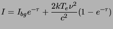
From the point of view of radio study of SNRs, the important point to note is that thermal emission progressively diminishes at frequencies below $\sim1$ GHz while the non-thermal emission progressively becomes stronger in this range of frequencies. Strong emission from H II regions has been observed all along the Galactic plane. High frequency observations close to or above this frequency are more sensitive to thermal emission and not well suited to the study of SNRs which emit non-thermal radiation at radio bands. On the other hand, at lower frequencies, thermal emission is diminished while non-thermal emission from SNRs progressively becomes stronger (see Fig. 5.15). Low frequency observations, where the contamination from thermal emission is minimized, are therefore more suited for the study of SNRs.

As mentioned above, angular resolution is important from the point of view of SNR identification and other detailed studies (particle acceleration, interaction with the local ISM, brightness variation as a function of galactic latitude, etc.). Since emission in the galactic plane occurs at all angular scales, it is also important that the observations be sensitive to large scale emission. To meet the requirement of high angular resolution with sensitivity to large scale emission, many observations of SNRs have been done at high frequencies either single dish instruments (Clark et al.1975b; Duncan et al.1997b; Clark et al.1975a; Duncan et al.1997a) or using interferometric telescopes (Gray1994b; Gray1994a; Kesteven & Caswell1987; Whiteoak & Green1996). However the uv-coverage of these interferometric observations was not good resulting into severe artifacts in the images. Also, these observations often suffer from contamination by thermal emission, particularly for fields in the Galactic plane.

The GMRT, operating at 150, 233, 327, 610 and 1400 MHz provides frequency coverage where, typically, non-thermal emission is dominant. With a shortest physical antenna separation of $\sim 100$ m and largest separation of $\sim25$ km, it also provides high angular resolution at these low frequencies ($\sim 20$ arcsec to $\sim2$ arcsec) while remaining sensitive to emission at large angular scales ( $\sim1{^\circ}$ to $\sim10$ arcmin). With a large collecting area, GMRT offers many advantages for the study of Galactic non-thermal emission in general and SNRs in particular. High resolution multi-frequency mapping of the galactic plane will also make it possible to identify compact sources of non-thermal emission (possibly compact SNRs) which may be confused with compact thermal sources in high frequency observations.

Radio morphology

The gross morphology of SNRs is largely governed by (1) properties of the progenitor and the pre-supernova circumstellar environment and (2) properties of the local interstellar medium and magnetic field. Traditionally, Galactic SNRs are classified in four different categories namely (1) shell-type, (2) filled centre (or Crab-type), (3) composite and (4) barrel shaped. About 80% of the SNRs in the Galactic SNR catalogue compiled and maintained by Green (2000) exhibit what is referred to as the shell-type morphology. This is expected from the generic model of an isotropic blast wave ploughing though the ISM and producing a bubble of emission after it slows down, having gathered enough ISM mass at the shock front. In projection, the bubble appears as a ring or shell of emission. On the other hand Crab-type SNRs exhibit a nebula of flat spectrum emission and is believed to be powered by the central neutron star. Variations of these basic morphologies are produced either due to a difference in the progenitor or in the local interstellar environment. The observed properties of these classes of SNRs are also therefore characteristic of the class and are briefly described below.

• Shell-type

  As mentioned above, 80% of the known Galactic SNRs are of this type. Typical examples are Kepler's and Tycho's SNR, SN 1006 (Fig. 1.4). These SNRs are characterized by a ring of emission which is often incomplete. As the blast wave decelerates, it enters the radiative phase of its evolution. The contact discontinuity between the shock front and the shocked medium is unstable and produces a thin shell of turbulence. The turbulence in the shell is believed to be the source of particle acceleration within the shell and magnetic field amplification by turbulent mixing (Chevalier1982). A reverse shock develops just behind the shell and moves into the out-flowing ejecta, heating it to sufficiently high temperatures to produce the observed X-ray emission (Chevalier & Fransson1994).

  Figure 1.4: Image of a typical Galactic Shell-type SNR SN 1006 (courtesy of ADIL; image code 98.BG.01.07). This 8-GHz image was made using the Molonglo Synthesis Radio Telescope (MOST). The brightened shell of emission with a weaker emission projected against the center is clearly seen.

  

  The typical average spectral index $\alpha$ along the shell ranges from $-0.7$ to $-0.3$. In some of the sensitive images of shell-type SNRs, weak emission (from the bubble) is sometimes seen in projection, filling the interior of the ring. The spectral index of this emission and the ring is, however the same, indicating that this corresponds to the bubble of emission seen projected at the centre of the shell. Substantial variation in the brightness across the shell of emission is often seen and may be due to the inhomogeneity of the local ISM with which the shock front interacts. This also produces spectral index variations in some cases (Anderson & Rudnick1993) indicating sites of enhanced particle acceleration or magnetic field amplification. The emission from the shell is linearly polarized at $5-15\%$ level and the inferred projected magnetic field is usually radial.

• Filled centre/Crab-like/Plerionic

  These types of SNRs are characterized by a flat spectrum plerionic emission ( $\alpha \ge -0.3$) almost uniformly filling the emission region. Less than 10% of the known Galactic SNRs are of this type. Strong linear polarization up to 30% level has been observed from such SNRs. A typical example of this class of SNRs, not surprisingly, is the Crab SNR (Fig. 1.5) or 3C58. Reynolds & Chevalier (1984) modeled a plerion as a spherical, homogeneous bubble of relativistic particles and magnetic field inflated by a central neutron star amidst uniformly expanding supernova ejecta. The plerionic emission is believed to be driven by the rotational energy losses of the central neutron star, which is seen as a pulsar at the centre of the Crab nebula. The central neutron star is believed to be the source of the magnetic field as well as of the energy which accelerates the electron in the medium thereby maintaining the flat spectrum of the emission. With the advent of high resolution X-ray telescopes, many plerionic SNRs have been found to be strong X-ray sources where the X-ray emission comes from the central region.

  Figure 1.5: Image of a typical Galactic plerionic SNR - The Crab nebula (courtesy of ADIL; image code 95.RP.02.01). This 327-MHz image was made using the VLA and is copyrighted by the NRAO^4.1(Observer: R.P.Perley). The compact source in the centre is the Crab pulsar.

  

  The blast wave should however produce a shell of emission outside such a nebula where it interacts with the ISM. The existence of a high-velocity, hydrogen-rich envelope corresponding to the initial blast wave is also required to account for the low total mass and kinetic energy of the observed nebula. No shell of emission has however been detected for such SNRs - at least not at radio frequencies. A deep search for the shell around the Crab nebula did not reveal any shell emission and this has been interpreted as being due to the blast wave expanding into a low density medium (Frail et al.1995). The spectral index of the plerionic emission for the Crab nebula is $\sim -0.26$. If the shell is close to the edge of the nebula, it can be distinguished from the nebula by the change in the spectral index from this value to close to $\sim -0.5$, typical for shock accelerated shell emission. No evidence for a significant change in the spectral index was found by these authors. Similarly no such shell has been found in H$\alpha$ and X-ray emission (Fesen et al.1997; Predehl & Schmitt1995). However, HST observations reveal a thin shell of [OIII] emission around the nebula (Sankrit & Hester1997) which is interpreted as a cooling region behind a radiative shock propagating at $\sim 150$ km s$^{-1}$ in a medium of density $\sim10$ cm$^{-3}$. Ironically, the Crab SNR may then no more be of the ``crab-type'' but may be re-classified as of the composite class (see below).

  Such shells have also not been detected for other plerionic SNRs. If the tenuous environment in which these SNRs are expanding is the reason for non-detection of the shell in radio continuum emission, it has been suggested that one must look for signs of interaction with the surrounding atomic or molecular gas (Jones et al.1998). 21-cm neutral hydrogen observations of G074.9+1.2 (CTB87), which is a pulsar powered SNR with no outer shell, shows that this SNR lies within an expanding HI bubble (Wallace et al.1997). The radio continuum emission also shows signs of flattening at a point of apparent contact between the HI bubble and the SNR, lending further support to this model. However evidence for a shell of emission around other plerionic SNRs like 3C58 remains elusive.

  Compact radio quiet thermal X-ray sources within SNRs have also been found in a few remnants (Gotthelf et al.1997; Vasisht & Gotthelf1997; Gotthelf & Vasisht1997). These compact objects may be radio quiet neutron stars in the SNRs and may thus explain the embarrassing lack of pulsar-SNR associations (Kaspi1998) in the sense that a non-pulsar neutron star or radio-quiet pulsar may be associated with many SNRs. The recent discovery of X-ray pulsations from some of these compact sources (Vasisht et al.2000; Gotthelf et al.2000) lend support to the idea that for these compact objects are indeed the elusive radio quiet neutron stars which are thought to be produced by the explosion and hence associated with the SNRs.

• Composite

  Figure 1.6: Image of a typical Galactic composite/mixed morphology SNR G000.9$+$0.1 taken from LaRosa et al. (2000). The shell and plerionic emission is clearly visible. The central compact source coincides with a compact thermal X-ray source.

  

  This class of SNRs exhibit characteristics of both shell-type and plerionic SNRs (Fig. 1.6). These SNRs are characterized by flat spectrum emission from the central region with a steeper spectrum shell of emission. Typical examples of this class of SNRs are G000.9$+$0.1, CTB80, G326.3$-$1.8.

  With high resolution imaging now possible in the X-ray band, this class has grown to include what are referred to as ``centrally influenced'' remnants; e.g. objects with shock powered radio shells with centrally enhanced X-ray emission. The X-ray radiation can be in the form of hard X-ray non-thermal emission from a compact nebula and/or extended soft thermal X-ray emission. Rho & Petre (1998) term SNRs with thermal X-ray emission inside hollow radio shells as ``mixed morphology'' SNRs. The X-ray emission is proposed to come from the evaporation of clouds (of pre-explosion origin) by the reflected and reverse shocks. Many of the thermal X-ray composite SNRs are interacting with molecular clouds (conclusions drawn from molecular line and OH maser observations, e.g. W44, 3C391, W28, IC443) (Frail et al.1994; Frail & Mitchell1998; Claussen et al.1997; Yusef-Zadeh et al.1999) and it has been suggested that this may be a generic property of the class.

• Barrel shaped

  Figure 1.7: Image of a typical Galactic barrel-type G003.7$-$0.2 (Gaensler1999) (image courtesy of ADIL; image code 98.BG.01.01). This 1.4-GHz VLA image shows the double arc structure with an axis of symmetry running right through the middle of the two brightened arcs of emission.

  

  These remnants are characterized by a clear axis of symmetry with lower emission along the axis in between two brighter limbs (Kesteven & Caswell1987; Caswell et al.1989; Whiteoak & Gardner1968) (Fig. 1.7). Proposed explanations for such a morphology are either on the lines of ``extrinsic'' effects relating to the ambient ISM and magnetic field and ``intrinsic'' effects relating to the progenitor and its circumstellar medium. Such morphologies can be produced if the ejecta expands inside an elongated cavity (Bisnovatyi-Kogan et al.1990). Alternatively, ejecta expanding in a uniform magnetic field will preferentially compress where the shock normal is perpendicular to the field lines producing enhanced emission where the magnetic field is more compressed (van der Laan1962). On the other hand, such morphologies can be produced due to intrinsic reasons like toroidal distribution of ejecta (Bodenheimer & Woosley1983) or due to initial high velocity of the progenitor (Rozyczka et al.1993) or intrinsic preferentially polar outflows from the central compact object (Manchester & Durdin1983; Willingale et al.1996).

  Analysis of highly resolved images of 17 barrel shaped SNRs done by Gaensler (1998) show evidence of a statistically significant tendency for the bilateral axes to be aligned with the Galactic plane. This is interpreted as lending support for the extrinsic effects being the dominant cause for the observed morphology - namely the alignment of the magnetic field with the Galactic plane.

Galactic distribution

Figure 1.8: Distribution of known Galactic SNRs as a function of Galactic longitude. Most of the known SNRs are in the 1st and 4th quadrants. The number of SNRs in the 4th quadrant are however slightly less than that in the 1st quadrant. Significant lack of SNRs in the 3rd and 2nd quadrants is attributed to lack of star forming regions there.

Fig. 1.8 shows the distribution of the known Galactic SNRs as a function of Galactic longitude. Most of the known Galactic SNRs are in the 1st or the 4th quadrant. This bias towards the inner Galaxy is attributed to the fact that most of the star forming regions are in the Galactic arms which cover a larger fraction of the inner Galaxy. However, there appears to be a mild lack of SNRs in the 4th quadrant compared to the 1st quadrant which is most likely to be due to some selection effect, probably due to the use of different telescopes in these quadrants (Gray1994b; Clark et al.1975b; Altenhoff et al.1979; Kesteven & Caswell1987; Duncan et al.1997b; Clark et al.1975a; Duncan et al.1997a; Whiteoak & Green1996; Gray1994a).

The incompleteness of the current Galactic SNR catalogue has been pointed out by Green (1991). He noted that the catalogue is incomplete in very large low surface brightness as well compact small sized young SNRs. Low surface brightness SNRs may be missed due to sensitivity limits of the observations. Higher frequency observations may also miss them because they are also inherently weaker at high frequencies. Such SNRs will also be missed in interferometric observations which are not sensitive to emission at angular scales larger than a maximum value. Small sized compact SNRs may be missing because of confusion with compact source of thermal emission. Any statistical result based on the current SNR catalogue is therefore likely to be affected by these selection biases. This is reflected in about a factor of $2-3$ error in the distance estimates for SNRs using the statistically derived $\Sigma$-$D$ relation. Green (1991) also argues that the proposed $\Sigma$-$D$-$z$ relation is not statistically significant.

Statistical studies of a complete sample of Galactic SNRs can help answer many question about the remnants themselves, their parent supernovae, their relation to pulsars and their interactions with the ISM and the ambient magnetic field. Observations to remove, if possible, the above mentioned biases in current catalogues are therefore important from the point of view of Galactic SNR research.

Effects of the ISM on the observed properties of SNRs

Most of the emission from SNRs is due to the interaction of the blast wave with the material into which it expands (the circumstellar envelope or the ISM). Low frequency spectral turnover, pulsar dispersion measures, HI absorption and brightness variations across SNRs, in particular along the shells of the shell-type SNRs suggest that the environments into which SNR expand are non-uniform. This is, however, hardly surprising since the structure and energetics of the ISM is largely dominated by star forming regions and supernova explosions, both of which are localized compared to the extent of the Galaxy. These density variations in the ISM are in-turn also expected to shape the morphologies of the SNRs. Interaction of the blast wave with higher density regions will result in stronger deceleration resulting in higher turbulence. This produces larger particle acceleration and consequently stronger synchrotron emission in such regions of interaction. On the other hand, the ejecta will expand at a more rapid rate in a lower density region and may even become radio loud at comparatively later times when the swept-up mass is enough to decelerate the blast wave. These effects are believed to give rise to the blow-out (G312.4$-$0.4), one-sided (G338.1$+$0.4) or irregular morphologies. The expanding blast also interacts with the ambient magnetic field and amplifies it via turbulent amplification or by simple compression of the frozen-in fields. This interaction of the blast wave with the magnetic field is believed to be responsible for the barrel shaped SNRs and it has been suggested that many intrinsically barrel shaped SNRs may not appear to be so due to projection effects (Gaensler1998).

Spatially resolved spectral index variations across SNRs trace changes in particle kinetic energies or magnetic field strengths or both. Both of these could also be due to the inhomogeneous nature of the medium into which the ejecta expands; reliable spatially resolved spectral index maps of SNRs thus give a handle on the scale of inhomogeneities in the ISM (Anderson & Rudnick1993; Katz-Stone et al.2000a). Spectral index changes across SNRs probe scales smaller than the size of the remnants. If the intrinsic properties of the SNRs can be independently established, spectral index changes between widely separated SNRs will probe scales of the order of the separation between the remnants.

It has been shown recently that the OH (1720 MHz) emission is associated with SNRs while the other OH maser transitions are associated with HII regions (Frail & Mitchell1998). Both theoretical and observational evidence (Reach & Rho1998; Reach & Rho1999; Frail & Mitchell1998) suggests that the OH (1720 MHz) masers are associated with the C-type shocks and are collisionally pumped in molecular clouds at temperatures and densities of $50-125$ K and $10^5-10^6$ cm$^{-3}$ respectively (Lockett et al.1999, and references therein). OH masers at 1665, 1667 and 1612 MHz cannot be produced under these physical conditions and the absence of these lines along with the detection of OH (1720 MHz) emission favors this interpretation. The measurements of the post shock density and temperature for IC443 (van Dishoeck et al.1993), W28, W44 and 3C391 (Frail & Mitchell1998) are in excellent agreement with these theoretical predictions. A solution to the problem of producing OH, which is not directly formed by shocks, are proposed by Wardle et al. (1999). They suggest that the molecular cloud is irradiated by the X-rays produced by the hot gas in the interior of the SNR. This leads to photo-dissociation of the H$_2$O molecules, which is produced by the shock wave in copious amounts, behind the C-type shock resulting in the required enhancement of OH just behind the shock. Indeed, such maser emission has been found in SNRs whose morphologies have long been suspected to be shaped by their interaction with nearby molecular clouds (Green et al.1997; Frail et al.1994; Claussen et al.1997). The fact that OH (1720 MHz) emission is possible for a very narrow range of physical parameters of the gas and other OH transitions in this range do not produce maser emission provides a powerful tool to probe the interaction of SNRs with molecular clouds. Detection of extended OH (1720 MHz) emission along with compact maser spots, tracing the radio continuum emission is suggestive of the maser emission tracing the extended region of such an interaction (Yusef-Zadeh et al.1999).

Why low frequency?

As mentioned above, radio emission from SNRs is synchrotron radiation which has a non-thermal power law dependence on frequency with a negative spectral index $\alpha$ ( $S \propto\nu^\alpha$). This makes the emission progressively stronger at lower frequencies (see Section 1.1). Thermal emission from typical HII regions, on the other hand has a flat spectrum above $\approx 1$ GHz. Below this frequency the optical depth is much greater than 1 and the spectrum turns over with a spectral index of 2. Continuum spectra of Galactic objects at low frequencies are therefore frequently used to distinguish between thermal and non-thermal sources of emission (Kassim & Weiler1990; Kassim et al.1989a; Subrahmanyan & Goss1995). Radio emission from SNRs is typically also extended, often with low surface brightness, with most of the remnants exhibiting easily identifiable morphologies. Detection of extended non-thermal emission in the Galaxy, with no thermal emission, has been the criterion used to identify Galactic sources as SNRs. Low frequency observations of SNRs also provide an added advantage in the sense that the surface brightness of typical SNRs increases at low frequencies, making it easier to detect and map them for detailed studies.

Interferometric telescopes are however insensitive to scales larger than those corresponding to the smallest projected baseline. Single dish telescopes, on the other hand, are sensitive to emission at all scales in the field. However, they provide the sensitivity and required resolution only at high frequencies. Many observations of SNRs till recently were therefore done using single dish instruments at high frequencies. However, apart from the contaminating thermal emission at these frequencies as well as inherently lower emission from SNRs, such observations are more prone to large scale confusing emission, which is abundantly present in the Galactic plane. The resolution of low frequency single dish observations is also not enough to resolve the extended emission.

Although high resolution interferometric observations of Galactic SNRs have been carried out, imaging at low frequencies using interferometers is also relatively tougher due to the problems arising from higher level of radio frequency interference (RFI), higher phase noise at low frequencies (due to various reasons ranging from cross talk to ionospheric phase corruption), non-co-planarity of arrays requiring much more complex software and higher computing power, etc. Hence, even interferometric observations have been typically done at frequencies $>1$ GHz.

Sensitive low frequency observations which are also sensitive to extended emission are therefore most appropriate for SNR research. Aperture synthesis telescopes like the GMRT operating at relatively low frequencies are well suited for such observations.

Aperture synthesis at low frequencies

Low frequency aperture synthesis telescopes like the GMRT offer several unique advantages from the point of view of SNR research. The GMRT is best suited for SNR observations owing to its sensitivity, relatively high resolution as well as sensitivity to large scale emission at low frequencies. Observations done for this dissertation extensively used the GMRT which has only recently come to a stage where enough antennas are available in the interferometric mode to attempt the imaging of extended sources. Interferometry at low frequencies, however, poses new challenges in data calibration and analysis, which are interesting in their own right. A substantial fraction of the work done for this dissertation involved the debugging and calibration of the telescope, to enable the observations discussed above to be carried out. Further, large amounts of software were required to be written, both to carry out debugging activity as well as to enable flagging and calibration of telescope data in a semi-automated fashion. The origin of the problems in low frequency interferometry and the required on-line data monitoring and off-line data analysis are briefly described below.

Phase fluctuations

The plasma frequency of the ionosphere is $\sim 12$ MHz. The only cosmic radio emission reaching the surface of the earth is at frequency significantly higher than this value. However radio observations at a few 100 MHz are still severely affected by the ionosphere. The ionosphere is modeled as a thin (compared to the distance from the observing plane) slab of inhomogeneous plasma. A plane wave incident on the ionosphere filled with plasma blobs will emerge with the plasma fluctuations imprinted on the phase of the wavefront (Fig.1.9). The amplitude of this wave front will remain largely unchanged but the phase is no longer constant. The RMS phase fluctuations of the visibility phase induced due to the Earth's ionosphere can be written as (Cronyn1972; Thompson et al.1986, and references therein)

Figure 1.9: Schematic diagram showing the effect of the ionosphere. The incident plane wave above the ionosphere is shown with a constant phase. The ionosphere, modeled as a thin slab of inhomogeneous plasma, imprints the inhomogeneities on the phase of the emergent wave front. The emergent corrugated wave front is sampled at a various points on the observing plane by antennas separated in space.

$$\Delta \phi = r_e \lambda a {\Delta N_e}$$ (4.20)

where $\lambda$ is the wavelength, ${\Delta N_e}$ is the fluctuation in the electron number density, $r_e$ is the classical electron radius and $a$ is the characteristic size of the blobs. Low frequency observations are therefore more severely affected by temporal and spatial fluctuations in the ionospheric electron content. The diurnal and seasonal temporal fluctuations in the ionospheric electron content induced by the Sun and Solar activity directly affect the phase measured by low frequency interferometers, which, if not corrected, affects the sensitivity of the observations. Spatial fluctuations in ${\Delta N_e}$ are at scales ranging from several kilometers up to hundreds of kilometers. The wave front emerging out of such a phase screen can be thought of as composed of a number of plane waves traveling in slightly different directions. Decomposing this resultant wave into an angular spectrum of plane waves arriving from a variety of angles, one can define a full width of the angular spectrum, $\theta_s$. This can be estimated by imagining that the blobs refract the incident wave by the amount $\pm\Delta \phi \lambda/2 \pi$ over a distance $a$. Thus,

$$\theta_s = \frac{1}{\pi} r_e \lambda^2 {\Delta N_e}\sqrt{L/a}$$ (4.21)

where $L$ is the thickness of the ionospheric plasma screen. Let the correlation length of the ionospheric phase fluctuation be $d$. Phase corruption from two points in the ionosphere separated by more than this amount will be uncorrelated. Assume further that the joint probability distribution of these phases is Gaussian with a variance of $\Delta \phi^2$ and a normalized correlation function given by $\rho(d)$. For the sake of better understanding, let us also assume that

$$\rho(d) = e^{-d^2/2a^2}$$ (4.22)

It can then be shown that for $d \ll a$, the expectation value of the measured visibility $V_m$ is given by

$${\langle}V_m {\rangle}= V e^{-\Delta\phi ^2 d^2/2a^2}$$ (4.23)

This limit samples the fluctuations in the phase due to fluctuations at length scales smaller than the typical blob size. Fluctuations at this scale induces small phase changes in the emerging wave front which can be treated as phase perturbations across the wavefront with the mean phase still preserved. Electron density fluctuations for $d > a$ induces large changes in the mean phase equivalent to a much larger spread in the angular spectrum. Consequently, ${\langle}V_m {\rangle}$ rapidly decreases for $d > a$.

The result of the these fluctuations is that a point source is broadened into a gaussian of diameter given by

$$\theta_s = \frac{\sqrt{2\ln 2}}{\pi} r_e \lambda^2 {\Delta N_e}\sqrt{L/a}$$ (4.24)

The final effect of phase fluctuations is therefore to effectively spread the power from a point source in the image (Cronyn1972). If the intrinsic resolution of the telescope is smaller than $\theta_s$, its resolution will be limited by the fluctuations in the phase and will be defined by $\theta_s$. A more realistic treatment involves a power-law spectrum of phase fluctuations, similar to the Kolmogorov model for turbulence in a neutral medium. With such a power-law model for phase fluctuations, it can be shown that $\theta_s\propto\lambda^{2.2}$.

Ionospheric electron density also changes as a function of time due to diurnal and seasonal changes in the position of the Sun and also due to the activity on the Sun. Since the induced phase fluctuations scale with the wavelength, the effect of ionosphere is more severe at low frequencies. These phase errors need to be calibrated before the measured visibilities can be used for mapping. Long term (several tens of minutes) variations in the phase of an interferometer can be measured by periodic observation of a source of known structure, usually referred to as the phase calibrator, using the self-cal algorithm which decomposes the visibility phases into antenna based phases (Cornwell & Wilkinson1981; Pearson & Readhead1984; Thompson & D'Addario1982). However for this, it is assumed that the variations in phase are small at angular scales smaller than the size of the primary beam of the antennas (iso-planatic case). At low frequencies, this assumption can break, at least for some fraction of time, and the derived phase corrections will not correct for the phase noise completely over the whole field. Schwab (1984) and Subrahmanya (1989) have described methods to relax the iso-planatic assumption. However, such algorithms have never been tried in real life or demonstrated to work well. This remains a potential problem, at least for high dynamic range imaging at low frequencies.

Non-coplanar baselines

The calibrated visibility function measured by an aperture synthesis telescope is given by^4.2

$$V(u,v,w)=\iint I(l,m)P(l,m)e^{-2\pi\iota (ul+vm+w(\sqrt{1-l^2-m^2}))} {dldm \over \sqrt{1-l^2-m^2}}$$ (4.25)

where $(u,v,w)$ are the projected co-ordinates of the antennas, $l,m,$ and $n$ are the direction cosines in the $uvw$ co-ordinates system, $I(l,m)$ is the source brightness distribution (the image) and $P(l,m)$ is the far field antenna reception pattern (the primary beam).

For a small field of view ( $l^2+m^2 \ll 1$), $V$ is related to the image by a 2D Fourier transform. However for $\theta_{PB}/\sqrt{\theta_r} > 0.1^{rad}$ where $\theta_{PB}$ and $\theta_r$ are the widths of the primary beam and the telescope resolution element, the image plane can no longer be expressed as a 2D Fourier transform of the visibility function (Cornwell & Perley1999). The sky can no longer be approximated by a 2D plane and must be modeled as the surface of a sphere, referred to as the Celestial sphere. To continue to approximate Equation 1.25 as a 2D Fourier transform relation between the sky brightness distribution and the visibility will introduce severe distortions in the image away from the phase centre. The longest baseline for the GMRT at 327 MHz is $\sim25$ km. Imaging with the GMRT at 327 MHz using baselines longer than $\sim 2-3$ km crosses the limit where the sky can be approximated, and a full 3D treatment of the problem is required to make distortion free images.

This problem can be handled by treating $\sqrt{1-l^2-m^2}$ as an independent co-ordinate. Re-writing Equation 1.25 as

$$V(u,v,w)=\iiint F(l,m,n)P(l,m)e^{-2\pi\iota (ul+vm+wn))} dldmdn$$ (4.26)

a full 3D Fourier transform of $V$ can then be used to make what is referred to as ``image volume''. $I$ can be shown to be related to $F$ as

$$F(l,m,n)={I(l,m)\delta(\sqrt{1-l^2-m^2}-n) \over {\sqrt{1-l^2-m^2}}}$$ (4.27)

where $\delta$ is the Dirac delta function. The 2D sky brightness distribution can be recovered from this image volume (Cornwell & Perley1992). This method goes by the name of ``3D inversion''. Alternatively, the sky can be approximated as a set of 2D tangent planes. Images can be made for points close to the tangent points of these planes using the 2D approximation. These images can then be properly combined to recover the full primary beam image of the sky. This method goes by the name of ``polyhedron imaging''.

The Galactic plane at low frequencies exhibits complex emission all over the field of view. Hence, even if the source of interest is compact and close to the pointing centre, 2D imaging cannot be applied since the distortions of sources away from the pointing centre (which is assumed to be also the phase centre) will have unacceptable effects all over the image. It is therefore necessary to map the full field of view, even if the size of the source of interest is small compared to the primary beam. Polyhedron imaging is implemented in the Astronomical Image Processing System (AIPS) package and was extensively used for making full primary beam images this dissertation.

On-line and off-line data analysis

In these early days of the GMRT, apart from other sources of data corruption like radio frequency interference (RFI), ionospheric scintillation, etc., data was frequently corrupted due to the failure of various systems. Monitoring the data quality and the health of the system during the observations was therefore of paramount importance. Since there were many sources of data corruption and the manner in which they affected the data were varied, it is useful to develop techniques and software which can automatically identify as many of these problems as early on in the data analysis process as possible. Identifying sources of data corruption, general debugging of the instrument, etc. however require sophisticated and efficient software for data analysis, browsing, and display. Extensive software was developed for this purpose in the form of general purpose object oriented libraries as well as programs for on-line and off-line data processing and display.

The effort invested in software development is optimally used if the resultant software is easy to use at the user level and easy to extend at the programmer level. This is also almost necessary for software which is expected to be used by a relatively larger number of users. Development of a user interface which is easy to use as well designing the entire software such that it is easy to extend is therefore important. Also, a user interface which is not consistent with the functionality of the application programs to which it interfaces is unlikely to be useful. It is therefore desirable to develop a user interface which, as far as possible, automatically evolves with the application programs. The modern Object Oriented software design philosophy was adopted to achieve exactly this goal. Software designed in an Object oriented manner is highly modular and the modules are loosely coupled. The software is designed as set of ``objects'' which map closely to real-life objects in the problem being solved. Usually, these real-life objects do not change significantly over the software life time, but the coupling between various objects can drastically change. Such changes can be very easily incorporated in a big software system designed as set of objects. Apart from ease of maintenance, this also produces reliable software which is easy to debug.

A user interface, which becomes part of the compiled application programs (as against a user interface as an independent entity which loads and runs the applications programs) was developed in the form of a set of libraries. Such a user interface is referred to as an embedded user interface. Libraries which provide a high level, astronomically useful interface for manipulating the GMRT visibility database were also developed. Using these libraries, programs for data editing, semi-automatic data flagging, on-line monitoring of the data, computation for antenna-based complex gains, amplitude and phase calibration, etc. were also developed.

The visibility function $V$, depends on a number of telescope parameters like the system temperature ($T^{sys}$), antenna sensitivity, antenna fixed delays, antenna positions, etc. For debugging as well as for on-line data monitoring, it was frequently required to extract this data in various representations (e.g., Cartesian versus polar representation of complex numbers). Since the complex visibilities are a function of a multitude of parameters, and different debugging purposes require viewing $V$ with respect to various quantities, it was necessary to develop a compact macro language parser to extract and display the data in a flexible and programmable manner. This macro language was implemented in the form of stand alone libraries as well as an application program which was extensively used for this dissertation.

The self-cal algorithm can be used to compute antenna based complex gains from the complex visibilities for a source of known structure. However, it is very sensitive to the presence of data from malfunctioning antennas or from a malfunctioning correlator. During the course of the observations, it was frequently the case that the data from a few antennas was unusable, at least for some fraction of the observing time. A large fraction of diagnosis of problems in the data/telescope is often done by examining the antenna based complex gains, which are computed using the self-cal algorithm which in turn required careful flagging of malfunctioning antennas/baselines. An algorithm was therefore implemented which was robust in such conditions and could identify bad baselines/antennas automatically. This was done by (1) automatically eliminating out-lying points, (2) doing two passes to eliminate dead/bad antennas. This algorithm was also used to identify and flag corrupted data in a semi-automatic fashion.

Instrumental polarization leakage

Signals from the two orthogonally polarized feeds are brought to the base of the antenna via co-axial cables, which run physically close to each other. These signals are then brought to the a central location via optical fibers where they are converted to baseband signals. The two orthogonally polarized signals can leak in each other at various points in the signal path resulting into polarization impurity. To minimize this leakage, the technique of Walsh switching (Thompson et al.1986, and references therein) is used wherein the two signals are multiplied by two orthogonal trains of square waves, called the Walsh functions. Later, before correlating the signals from different antennas, these Walsh switched signals are multiplied by the inverse Walsh functions to recover the original signals. Any leaked signal from one polarization channel to the other at time scales longer than the period of the Walsh functions then averages to zero.

The planned Walsh switching has not yet been implemented for the GMRT. In any case, polarization impurity introduced before the switching point will not be removed by Walsh switching. This leakage is a significant source of noise at 150 MHz and also contributes noise at all other bands, albeit at a lower level and manifests itself in the form of increased closure errors in the system (Rogers1983). The current GMRT correlator computes only the co-polar visibilities (i.e. RR and LL visibilities only). Even with the planned extension of the correlator where the cross-polar visibilities (i.e. RL and LR visibilities) will also be computed, one can think of observations which will be done using the higher frequency resolution provided by the GMRT correlator in the non-polar mode. All such data will then be affected by errors related to this polarization impurity related errors. Rogers (1983) pointed out in the context of the VLBA, that polarization leakage causes closure errors even in nominally co-polar visibilities. Massi et al. (1997) have carried out a detailed study of this effect for the telescopes of the European VLBI Network (EVN). The polarization leakage in some of the EVN antennas corrupts the co-polar visibilities at a level visible as a reduction in the dynamic range of the maps (Massi & Aaron1997a; Massi & Aaron1997b; Massi et al.1998).

Non-polarimetric observations for imaging constitute a large fraction of observations done using interferometers where only the co-polar visibilities are recorded. The calibrators used for such observations are usually unpolarized. Since the above mentioned closure errors will affect such data adversely, a method to measure the polarization leakage using only the co-polar visibilites from an unpolarized calibrator to correct for these closure errors will be of use, particularly for high dynamic range imaging.

Organization of the thesis

Low frequency continuum spectra, radio morphology and, if possible polarization measurements are the key observables used to identify SNRs in the Galaxy. Spectra at frequencies greater than $\sim1$ GHz suffer from contaminating thermal emission. Therefore, although higher angular resolution observations can be done at high frequencies, low frequency radio observations are more suited for SNR research. However with the lower resolutions and sensitivities at low frequencies, identification of the morphology, particularly in regions with complicated emission becomes difficult. High resolution sensitive observations at low radio frequencies therefore appears to be the optimal observation expected to yield rich dividends for various aspects of SNR research. This thesis reports the work done on these lines using the GMRT.

The main thrust of the thesis is the study of Galactic SNRs taking advantage of the high sensitivity and resolution of the GMRT which has recently become available for scientific usage. Since this work was done in the early stages of the GMRT, a large fraction of time was also spent in debugging the instrument and in developing extensive software for data browsing, display and off-line analysis. New algorithms and techniques were also developed which were useful, in particular for the GMRT, and, in general, for low frequency interferometry.

While debugging the GMRT, need for a sophisticated software for data browsing, display and analysis was felt early on. As a result, large amounts of software ($>60 000$ lines of code in C++, C and FORTRAN) was written with the goal of keeping it efficient and yet simple so that the turn around time between observations and results from data analysis is minimized. This software was also written in a modern object oriented fashion, with the hope that many more astronomers/engineers will find it useful to write useful application programs using the the underlying software libraries as well as to extend the software system.

The thesis is organized in the form of eight chapters and four appendices. The present chapter briefly describes the model for supernova explosions and introduces the theoretical concepts of radio synchrotron emission in Section 1.1. Particular emphasis is laid on the fact that low radio frequency observations for the purpose of identification of SNRs in the Galaxy provides a crucial advantage over high frequency observations. The various stages of the evolution of SNRs are described in Section 1.2. Proposed mechanisms to explain the observed non-thermal emission from SNRs are discussed in Section 1.2.1 and the information drawn from measured continuum spectra of SNRs is discussed in Section 1.2.2. At frequencies higher than $\sim1$ GHz, thermal emission from HII regions in the Galaxy is strong and sometimes even dominant. The spectral signatures and nature of thermal emission in the presence of absorbing foreground medium are discussed in Section 1.2.3. Various observed radio morphologies, distribution of SNRs in the Galaxy and the effects of the ISM on the observed properties of SNRs are discussed in Sections 1.2.4, 1.2.5 and 1.3 respectively.

Chapter 2 describes the GMRT from an astronomical point of view. The underlying principle of aperture synthesis is discussed in Section 2.1, with emphasis on the problems related to imaging at low frequencies. Section 2.2 briefly describes the parabolic dishes and the geometry of the array. Section 2.3 describes the signal path from the antennas feeds till the digital back-end correlator while Section 2.4 describes the astronomically relevant parameters of the telescope. Most of the observations included in this dissertation were done when the GMRT hardware as well software was in a state of being debugged. Consequently, a large fraction of the time was spent in debugging activities, which required understanding the details of the hardware - particularly of the GMRT FX-type correlator. The GMRT correlator hardware and associated software is described in some detail in Section 2.5. Section 2.5.1 describes the algorithm used for accurate time stamping of the data in the data acquisition software. Precise location of the antennas on the ground as well as the fixed instrumental delay suffered by the signal from individual antennas before reaching the correlator are two important parameters of an aperture synthesis telescope. Before imaging could be attempted, these measurements were made for the GMRT. Details of the baseline and antenna fixed delay calibration and its results are described in Section 2.6.

Chapter 3 very briefly describes the design and implementation of the GMRT off-line data analysis software system, which was extensively used during the course of this work. Section 3.1 discusses the need for the development of such a software system. Section 3.2 describes the philosophy behind the design of this software system consisting of a set of generic libraries and a number of application programs. Data manipulation libraries are described briefly in Section 3.3 while the user interface system and a few selected application programs, most extensively used during the course of this work, are described in Sections 3.4 and 3.5 respectively.

Chapter 4 describes the 325-MHz GMRT observations of a sample of candidate SNR fields. Section 4.1 describes the parameters of these observations. Mapping in the Galactic plane at 325-MHz with the GMRT requires mapping of the entire field of view which in turn requires use of specialized imaging and deconvolution algorithms. Section 4.2 discusses the techniques used from imaging at low frequencies, which were used for mapping the GMRT data. Section 4.3 describes the observational procedure used for these observations including the use of off-line data analysis software for on-line monitoring of the system health and the data quality. The details of data analysis and calibration are described in Section 4.4. Section 4.5 discusses the details related to inversion of the visibility data and deconvolution of the images. Finally, Section 4.6 presents the full primary beam 325-MHz images of all the fields. Most of the SNRs studied in this dissertation are large in angular size (typically $>7$ arcmin). Although these GMRT observations could provide typical resolution of $\sim 20$ arcsec for these southern fields, the maps presented here are typically at arcmin resolution. The reason for this is two fold: (1) since many of the SNRs had low surface brightness, lower resolution maps show the morphology more clearly (2) large scale emission tend to ``break-up'' at the highest resolution due to a combination of problems of deconvolution of large sources as well as phase noise that could not be calibrated. For a few fields, where the angular size of the sources of interest was of the order of arcmin, high resolution images were used.

Full primary beam maps of almost all the fields at 325-MHz exhibit a number of sources of compact as well extended emission, particularly in the Galactic plane. The primary goal of these observations was the low frequency study of Galactic SNRs in the fields - many of which were not confirmed SNRs. Chapter 5 goes on to discuss the SNRs in these fields. Section 5.1 discusses the difference between low and high frequency observations of Galactic SNRs to bring forth the advantages offered by deep high resolution observations at low frequency. Section 5.2 then discusses the individual candidate SNRs in the fields. Some of the fields also contained other previously identified SNRs. For a few of them, these 325-MHz observations are the first observations at this frequency; in fact, these are also the first high resolution observations at this frequency for all these sources. These results are described and discussed in Section 5.3. Finally, Section 5.4 discusses these results in a broader perspective of Galactic SNR research.

Other sources in the field are discussed in Chapter 6. Section 6.1 briefly discusses the nature of other dominant sources of radio emission and Section 6.2 presents a list of point sources in the fields along with their measured flux densities at 325-MHz and, where possible, at 1400 MHz. Section 6.3 discusses the sources of extended emission in these fields, which are not SNRs. These high resolution observations at relatively low frequency are the first ever observations of these objects and the somewhat unexpected significant extended emission seen at this frequency is interesting from the point of view of better understanding of these sources (usually classified as ``thermal''). Section 6.5 concludes the chapter with a summary of the results from these observations.

A technique for the computation of polarization leakage using only the co-polar visibilities is described in Chapter 7. Section 7.2 describes the motivation which led to the development of this technique. Section 7.3 mathematically describes the algorithm and also presents the results of the simulations done to test it. Section 7.4 presents the results of the tests done with real data acquired in a controlled experiment and the interpretation of the results in terms of the magnitude of the polarization leakage for various antennas. The Poincaré sphere is a convenient and possibly more intuitive representation of the polarization state of radiation. Interpretation of these results on the Poincaré sphere and the equivalence of the polarization leakage induced phase closure errors and the Pancharatanam phase is discussed in Section 7.5. Since only co-polar visibilities are used for the computation of polarization leakage, the solutions are not unique, but still provide useful information about the polarization properties of the antennas. This is discussed in Section 7.6.

Chapter 8 gives consolidated conclusions and results from this work. Section 8.1 describes the major results from the testing and debugging of the GMRT and the software developed for the purpose. Section 8.2 discusses the astronomical results from the observations of the candidate SNRs done for this dissertation. Section 8.3 discusses the inferences about other sources in the fields based on these low frequency observations. Section 8.4 proposes the future directions of research in the fields of Galactic SNRs, compact/Ultra compact H II regions as well as in the field of developing data analysis techniques for radio interferometry at low frequencies and related software development.

Details of the user interface for the off-line software is included as Appendix A. A flexible mechanism was developed to allow easy extraction for any type of data from the GMRT visibility database. This was implemented in the form of a macro language; and the parser and complier for this language is implemented as a stand alone library and used in the program xtract. Details of all this work are included as Appendix B. A flexible antenna and baseline naming convention is uniformly used in all off-line application programs. This convention is described in Appendix C. Finally, Appendix D presents the formulation of the problem of computation of antenna based complex gains from the measured complex visibilities. The iterative equations are derived using complex calculus and the interpretation of these equations for better understanding of the algorithm is also presented.