Recent Galactic plane observations at 843 MHz, using the Molonglo Synthesis Telescope (MOST) (Gray1994a) and at 2.4 GHz, using the Parkes 64-m single dish (Duncan et al.1997b), have revealed a number of new candidate SNRs. However many of these objects were in complicated regions of the Galaxy and these observations also suffered from contamination due to thermal emission at these high frequencies. Although the MOST observations were at a relatively low frequency, the side-lobes due to nearby strong sources severely limited the fidelity of images. With only single frequency data available for most of these fields (these observations did not have any overlapping fields), the identification of the candidate SNRs in these fields remained inconclusive.
A sample of candidate SNRs, accessible to the GMRT, were selected from these observations. Continuum observations of this sample were done with the GMRT at 325 MHz during the period of 1998 to 2000. The telescope hardware, on-line and off-line software were all in a state of being debugged during this period and observations were invariably intermingled with debugging activity and related observations. Consequently, the data acquired was often unusable, sometimes requiring several observing sessions involving the same field to get good data. This chapter describes the procedure used for on-line data monitoring and identification of a potential source of data corruption, off-line data flagging and finally imaging using the AIPS package.
Section 4.1 gives the general description of the observations done at 325 MHz. Imaging at these low frequencies requires the use of algorithms and techniques not usually used for mapping at higher frequencies. These low frequency specific problems for inversion of visibilities and image deconvolution, and the techniques used to overcome these problems are discussed in Section 4.2. Section 4.2.2 discusses the problem of bandwidth smearing of sources away from the phase centre, which necessitates the multi-channel mode of observations. The procedures used for on-line system and data monitoring are described in Section 4.3. The detailed procedure used for off-line data editing and calibration is described in Sections 4.4. Section 4.5 describes the procedure used to finally map the data and while Section 4.6 presents the full primary beam images after correcting for the primary beam attenuation.
325 MHz observations for continuum imaging of a sample of nine
candidate SNRs were done during the period of 1998-2000. The
parameters of these observations are summarized in
Table 4.1. Most of the objects of interest in these
fields were extended, with emission at angular scales
![]() arcmin requiring reliable observations at the smallest
available baselines. Observations at 325 MHz are often affected by
intermittent radio frequency interference (RFI) and, since RFI from
nearby sources of emission remains partially correlated for the
smallest baselines, data from the smallest baselines are also most
severely affected by RFI. Fortunately, RFI is often narrow band and
can be identified if the observing band is split into a number of
narrow band frequency channels. The observations were therefore done
with the full 16 MHz band split into 128 frequency channels of each
having a width of
arcmin requiring reliable observations at the smallest
available baselines. Observations at 325 MHz are often affected by
intermittent radio frequency interference (RFI) and, since RFI from
nearby sources of emission remains partially correlated for the
smallest baselines, data from the smallest baselines are also most
severely affected by RFI. Fortunately, RFI is often narrow band and
can be identified if the observing band is split into a number of
narrow band frequency channels. The observations were therefore done
with the full 16 MHz band split into 128 frequency channels of each
having a width of ![]() kHz.
kHz.
The current single side-band GMRT correlator measures only the
co-polar visibilities, i.e. only signals of the same polarization are
correlated using the Indian mode of the VLBA Multiplier and
Accumulator chips (MACs). All the 128 frequency channels of the
co-polar visibilities corresponding to the right and left circular
polarized signals were recorded for all available baselines. The data
was kept in the multi-channel format throughout the imaging process to
minimize the band-width smearing of sources away from the phase centre
(see Section 4.2.2). After editing the
RFI-affected or otherwise bad data, a typical bandwidth of about
![]() MHz was finally used for imaging giving a typical RMS noise of
MHz was finally used for imaging giving a typical RMS noise of
![]() mJy/beam.
mJy/beam.
The background sky temperature can vary by a factor of ![]() within
the Galactic plane, resulting in a change in the total power output by
similar factors. The correlator samplers are, however, optimized to
work with an input signal of 0 dBm. To keep the sampler inputs at
this level, automatic level controllers (ALCs) are introduced at
the output of the baseband (BB) which effectively changes the gain to
keep the output at 0 dBm. To keep the ALC operating point within its
linear operating range, an attenuation of 16 db was typically used for
the IF and BB signals.
within
the Galactic plane, resulting in a change in the total power output by
similar factors. The correlator samplers are, however, optimized to
work with an input signal of 0 dBm. To keep the sampler inputs at
this level, automatic level controllers (ALCs) are introduced at
the output of the baseband (BB) which effectively changes the gain to
keep the output at 0 dBm. To keep the ALC operating point within its
linear operating range, an attenuation of 16 db was typically used for
the IF and BB signals.
| Frequency of Observations (MHz) | 325 |
| RF Bandwidth (MHz) | 16 |
| Bandwidth used (MHz) | |
| Integration time (sec) | 16.9 |
| Average time spent on the source (hr) | 5 |
| No. of Antennas used | |
| Max. baseline (k |
|
| Min. baseline ( |
|
| Max. spatial scale(arcmin) | |
| Average Antenna Sensitivity (K/Jy) | 0.32 |
| Primary beam (degree) | 1.4 |
| Synthesized resolution (arcsec) | |
| RMS noise (mJy/beam) |
As mentioned earlier, the GMRT was in a state of being debugged during
the period of the observations. Consequently, the number of antennas
and the longest baseline available changed from observation to
observation. As a result, the resolution changes from observation to
observation. However, most of the Central Square antennas, plus some of the arm
antennas were available for all observations giving angular resolution
in the range
![]() arcsec. Some of the fields, which needed
higher resolution were observed when the long baselines antennas were
available. Since most of the target objects were extended, it was
essential that the short antenna spacings were well sampled. Hence
the three antennas, C05, C06 and C09 which provide the shortest
spacings, were used for all observations giving a shortest baseline of
arcsec. Some of the fields, which needed
higher resolution were observed when the long baselines antennas were
available. Since most of the target objects were extended, it was
essential that the short antenna spacings were well sampled. Hence
the three antennas, C05, C06 and C09 which provide the shortest
spacings, were used for all observations giving a shortest baseline of
![]() (after flagging bad data) for which reliable data was
measured. This corresponds to a largest angular scale of
(after flagging bad data) for which reliable data was
measured. This corresponds to a largest angular scale of
![]() arcmin. Most of the sources of interest were well within
this limit in angular size and we believe that most of the emission up
to angular scales of
arcmin. Most of the sources of interest were well within
this limit in angular size and we believe that most of the emission up
to angular scales of ![]() arcmin is well represented in the GMRT
325-MHz images.
arcmin is well represented in the GMRT
325-MHz images.
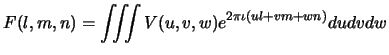
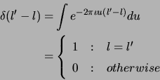
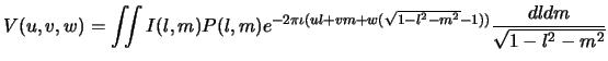
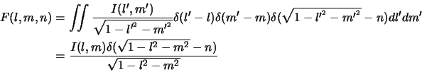
The visibility measured by a properly calibrated interferometer is given by
For a small field of view (
![]() ), the above equation can be
approximated well by a 2D Fourier transform relation. The other case
in which this is an exact 2D relation is when the antennas are perfect
aligned along the East-West direction. Here, we discuss the problem
of mapping with non-East-West arrays. The derivation presented here
of results for devising algorithms used for imaging large fields of
view presented here follow the treatment of
Cornwell & Perley (1992) and Cornwell & Perley (1999).
), the above equation can be
approximated well by a 2D Fourier transform relation. The other case
in which this is an exact 2D relation is when the antennas are perfect
aligned along the East-West direction. Here, we discuss the problem
of mapping with non-East-West arrays. The derivation presented here
of results for devising algorithms used for imaging large fields of
view presented here follow the treatment of
Cornwell & Perley (1992) and Cornwell & Perley (1999).
Equation 4.1 also reduces to a 2D relation for a non-East-West array, if the integration time is sufficiently small (snapshot observations). However modern arrays are designed to maximize the uv-coverage with the antennas arranged in a 'Y' shaped configuration (non East-West arrays) (Mathur1969). Fields, such as the ones observed for this dissertation, with emission at all angular scales, require maximal uv-coverage. Telescopes such as the GMRT use the rotation of earth to improve the uv-coverage and observations of complex fields typically last for several hours. Hence, Equation 4.1 needs to be used to map the full primary beam of the antennas, particularly at low frequencies.
Let
![]() be treated as an independent variable. A 3D
Fourier transform of
be treated as an independent variable. A 3D
Fourier transform of ![]() can be written using (
can be written using (![]() ) and
(
) and
(![]() ) as a set of conjugate variables as
) as a set of conjugate variables as
 |
(7.2) |
 |
 |
||
 |
|||
| (7.3) |
 |
(7.4) |
The effect of including the fringe rotation term (![]() ) would be
a shift of the Image volume by one unit in the conjugate axis
(
) would be
a shift of the Image volume by one unit in the conjugate axis
(![]() axis) (shift theorem of Fourier transforms; Bracewell1986and later eds).
Hence, the effect of fringe stopping is to make the
axis) (shift theorem of Fourier transforms; Bracewell1986and later eds).
Hence, the effect of fringe stopping is to make the ![]() plane coincide
with the tangent plane at the phase center on the Celestial sphere
(the point where the tangent plane touches the Celestial sphere) with
the rest of the sphere completely contained inside the Image
volume (Fig. 4.1).
plane coincide
with the tangent plane at the phase center on the Celestial sphere
(the point where the tangent plane touches the Celestial sphere) with
the rest of the sphere completely contained inside the Image
volume (Fig. 4.1).
![\includegraphics[scale=0.85]{Images/ImgVol.eps}](img576.png)
|
![\includegraphics[]{Images/CelestialProj.eps}](img577.png)
|
Noting that the third variable ![]() of the Image volume is not an
independent variable and is constrained to be
of the Image volume is not an
independent variable and is constrained to be
![]() ,
Equation 4.5 gives the physical interpretation of
,
Equation 4.5 gives the physical interpretation of ![]() .
Imagine the Celestial sphere defined by
.
Imagine the Celestial sphere defined by
![]() enclosed by
the Image volume
enclosed by
the Image volume ![]() , with the top most plane being
tangent to the Celestial sphere as shown in Fig. 4.1.
Equation 4.5 then tells that only those parts of the Image
volume correspond to the physical emission which lie on the surface
of the Celestial sphere. However, the Image volume will be
convolved by the telescope transfer function. The telescope transfer
function is the Fourier transform of the sampling function
, with the top most plane being
tangent to the Celestial sphere as shown in Fig. 4.1.
Equation 4.5 then tells that only those parts of the Image
volume correspond to the physical emission which lie on the surface
of the Celestial sphere. However, the Image volume will be
convolved by the telescope transfer function. The telescope transfer
function is the Fourier transform of the sampling function ![]() in the
in the
![]() frame (see Chapter 2,
page
frame (see Chapter 2,
page ![]() ). The telescope transfer function,
referred to as the dirty beam and defined as
). The telescope transfer function,
referred to as the dirty beam and defined as
![]() , also defines a volume in the image domain. The dirty image volume defined by the relation
, also defines a volume in the image domain. The dirty image volume defined by the relation
![]() is a convolution of
is a convolution of ![]() with
with ![]() . Since
the dirty beam is not constrained to be finite only on the
Celestial sphere,
. Since
the dirty beam is not constrained to be finite only on the
Celestial sphere, ![]() will be finite away from the surface of the
Celestial sphere corresponding to non-physical emission due to the
side lobes of
will be finite away from the surface of the
Celestial sphere corresponding to non-physical emission due to the
side lobes of ![]() . A 3D deconvolution using the dirty
image and the dirty beam volumes will produce a Clean
image volume. An extra operation of projecting all points in the
CLEAN image-volume along the Celestial sphere onto the 2D
tangent plane to recover the 2D sky brightness distribution is
therefore required. Graphical representation of the geometry for this
is shown in Fig. 4.1.
. A 3D deconvolution using the dirty
image and the dirty beam volumes will produce a Clean
image volume. An extra operation of projecting all points in the
CLEAN image-volume along the Celestial sphere onto the 2D
tangent plane to recover the 2D sky brightness distribution is
therefore required. Graphical representation of the geometry for this
is shown in Fig. 4.1.
The most straight forward method suggested by Equation 4.5 for
recovering the sky brightness distribution, is to perform a 3D Fourier
transform of ![]() . This requires that the
. This requires that the ![]() axis be also
sampled at the Nyquist rate (Bracewell1986and later eds; Brigham1988and later eds)). For most
observations, it turns out that this is rarely satisfied and doing a
FFT along the third axis would result into severe aliasing.
Therefore, in practice, the Fourier transform on the third axis is
usually performed using the direct Fourier transform (DFT) on the
un-gridded data.
axis be also
sampled at the Nyquist rate (Bracewell1986and later eds; Brigham1988and later eds)). For most
observations, it turns out that this is rarely satisfied and doing a
FFT along the third axis would result into severe aliasing.
Therefore, in practice, the Fourier transform on the third axis is
usually performed using the direct Fourier transform (DFT) on the
un-gridded data.
To perform the 3D FT (FFT along the ![]() and
and ![]() axis and DFT along
the
axis and DFT along
the ![]() axis) one still needs to know the number of planes needed
along the
axis) one still needs to know the number of planes needed
along the ![]() axis. This can be found using the geometry shown in
Fig. 4.2. The size of the synthesized beam along the
axis. This can be found using the geometry shown in
Fig. 4.2. The size of the synthesized beam along the
![]() axis is comparable to that along the other two directions and is
given by
axis is comparable to that along the other two directions and is
given by
![]() where,
where, ![]() is the longest
projected baseline length. The separation between the planes along
is the longest
projected baseline length. The separation between the planes along
![]() should be
should be
![]() . The distance between the tangent
plane and a point separated by
. The distance between the tangent
plane and a point separated by ![]() from the phase center, for
small values of
from the phase center, for
small values of ![]() , is given by
, is given by
![]() . For a field of view of angular size
. For a field of view of angular size ![]() , critical
sampling would be ensured if the number of planes along the
, critical
sampling would be ensured if the number of planes along the ![]() axis,
axis,
![]() , is
, is
Another reason why more than one plane would be required for very high
dynamic range imaging is as follows. Strictly speaking, the only
point which lies in the tangent plane is the point at which the
tangent plane touches the Celestial sphere. All other points in the
image, even close to the phase center, lie slightly below the tangent
plane. Deconvolution of the tangent plane then results into
distortions for the same reason as the distortions due to the
deconvolution of a point source which lies between two pixels in the
2D case (Briggs1995). As in the 2D case, this problem can be
minimized by over sampling the image which, in this case, implies
having more than one plane along the ![]() -axis, even if
Equation 4.6 implies that one plane is sufficient.
-axis, even if
Equation 4.6 implies that one plane is sufficient.
As mentioned above, emission from the phase center and from points close to it, lie approximately in the tangent plane. Polyhedron imaging relies on exploiting this by approximating the Celestial sphere by a number of tangent planes, referred to as facets, as shown in Fig. 4.3. The visibilities are recomputed to shift the phase center to the tangent points of each facet and a small region around each of the tangent points is then mapped using the 2D approximation.
The number of planes required to map an object of size ![]() can be
found simply by requiring that the maximum separation between the
tangent plane and the Celestial sphere be less than
can be
found simply by requiring that the maximum separation between the
tangent plane and the Celestial sphere be less than
![]() ,
the size of the synthesized beam. As shown earlier, this separation
for a point
,
the size of the synthesized beam. As shown earlier, this separation
for a point ![]() degrees away from the tangent point is
degrees away from the tangent point is
![]() . Hence, for critical sampling, the number of planes
required is equal to the solid angle subtended by the sky being mapped
(
. Hence, for critical sampling, the number of planes
required is equal to the solid angle subtended by the sky being mapped
(
![]() ) divided by
) divided by
![]() (
(
![]() )
)
 |
(7.7) |
The polyhedron imaging scheme is implemented in the current version of the AIPS data reduction package and the 3D inversion (and deconvolution) is implemented in the (no longer supported) SDE package developed by T.J. Cornwell et al. Both these schemes, in their full glory, are available in the (recently released) AIPS++ package.
The GMRT 325-MHz data was imaged using the IMAGR task in AIPS.
This program implements the polyhedron algorithm and requires the user
to supply the number of facets to be used and a list of the locations
of the centre of each facet with respect to the image centre and the
size of each facet. This list of facets and their parameters were
computed using the task SETFC in AIPS, typically resulting in a
grid of ![]() facets, each of size
facets, each of size
![]() pixels.
pixels.
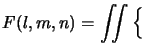
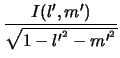
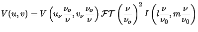
The effect of a finite bandwidth of observation as seen by the
multiplier in the correlator, is to reduce the amplitude of the
visibility by a factor given by
![]() where
where ![]() is the
angular size of the synthesized beam,
is the
angular size of the synthesized beam, ![]() is the center of the
observing band,
is the center of the
observing band, ![]() is location of the point source relative to the
field center and
is location of the point source relative to the
field center and
![]() is the bandwidth of the signal being
correlated.
is the bandwidth of the signal being
correlated.
The distortion in the map due to the finite bandwidth of observation
can be understood as follows. For continuum observations, the
visibility data integrated over the bandwidth
![]() is treated
as if the the observations were made at a single frequency
is treated
as if the the observations were made at a single frequency ![]() -
the central frequency of the band. As a result the
-
the central frequency of the band. As a result the ![]() and
and ![]() co-ordinates and the value of visibilities are correct only for
co-ordinates and the value of visibilities are correct only for
![]() . The true co-ordinates at other frequencies in the band are
related to the recorded co-ordinates as
. The true co-ordinates at other frequencies in the band are
related to the recorded co-ordinates as
| (7.8) |
 |
(7.11) |
The effect of bandwidth smearing can be reduced if the band is split
into frequency channels with smaller channel widths. This effectively
reduces the bandwidth ![]() as seen by the mapping procedure and
while gridding the visibilities,
as seen by the mapping procedure and
while gridding the visibilities, ![]() and
and ![]() can be computed
separately for each channel and assigned to the appropriate uv-cell.
The FX correlator used in GMRT provides up to 128 frequency channels
over the entire bandwidth of observation and the visibilities can be
retained as multi-channel in the mapping process to reduce bandwidth
smearing. Although purely from the point of view of bandwidth
smearing, averaging
can be computed
separately for each channel and assigned to the appropriate uv-cell.
The FX correlator used in GMRT provides up to 128 frequency channels
over the entire bandwidth of observation and the visibilities can be
retained as multi-channel in the mapping process to reduce bandwidth
smearing. Although purely from the point of view of bandwidth
smearing, averaging ![]() channels at 325 MHz would be
acceptable, keeping the visibility database with all the 128 channels
is usually recommended to allow identification and flagging of narrow
bands RFI.
channels at 325 MHz would be
acceptable, keeping the visibility database with all the 128 channels
is usually recommended to allow identification and flagging of narrow
bands RFI.
For
![]() , the amplitude of the visibility function
, the amplitude of the visibility function ![]() is
proportional to the flux density of the source and the normalized
visibility amplitude is converted to flux density units using the
measurement of
is
proportional to the flux density of the source and the normalized
visibility amplitude is converted to flux density units using the
measurement of ![]() for a source of known but non variable flux density
(referred to as the flux density calibrator). Also, the complex
antenna based gain can potentially vary as a function of time. These
slow time variations can be corrected using periodic observation of a
source of known structure, usually an unresolved source, referred to
as the phase calibrator. The flux density of the phase calibrators,
the flux density of which is potentially variable over time scales of
days, is also calibrated using the flux density calibrator. Each
observation therefore requires at least one observation of a flux
density calibrator and periodic observation of phase calibrators to
properly calibrate the data.
for a source of known but non variable flux density
(referred to as the flux density calibrator). Also, the complex
antenna based gain can potentially vary as a function of time. These
slow time variations can be corrected using periodic observation of a
source of known structure, usually an unresolved source, referred to
as the phase calibrator. The flux density of the phase calibrators,
the flux density of which is potentially variable over time scales of
days, is also calibrated using the flux density calibrator. Each
observation therefore requires at least one observation of a flux
density calibrator and periodic observation of phase calibrators to
properly calibrate the data.
The VLA flux density calibrators, 3C48 and 3C286 was used
for all observations. One of three calibrators close to the Galactic
plane namely, 1830-36, 1709-299 and 1822-096, were
used as the phase calibrator. A flux calibrator was observed for
![]() min at the beginning and at the end of each observing session
and the phase calibrator was observed for
min at the beginning and at the end of each observing session
and the phase calibrator was observed for ![]() min at an intervals
of
min at an intervals
of ![]() min.
min.
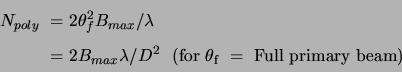
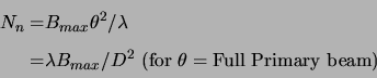
The planned periodic injection of noise from a calibrated noise source
to measure the system temperature has not yet been implemented for the
GMRT. As a result, the system temperatures for the flux density
calibrator fields (
![]() ) and the field being mapped
(
) and the field being mapped
(
![]() ) must be measured and a correction equal to
) must be measured and a correction equal to
![]() be applied as part of the flux density
calibration.
be applied as part of the flux density
calibration.
![]() was measured to be
was measured to be ![]() K while
K while
![]() was estimated from the all-sky maps at 408 MHz
(Haslam et al.1982; Haslam et al.1995; Haslam et al.1981). For a few fields,
was estimated from the all-sky maps at 408 MHz
(Haslam et al.1982; Haslam et al.1995; Haslam et al.1981). For a few fields,
![]() was also measured at few points around the source of
interest and the measured system temperature was consistent with that
estimated from the 408 MHz data to within
was also measured at few points around the source of
interest and the measured system temperature was consistent with that
estimated from the 408 MHz data to within ![]() . None of the
phase calibrators used for these observations are known to be variable
over few hours. These calibrators were therefore also used as
secondary amplitude calibrators to effectively correct for any slow
variation in the receiver temperature.
. None of the
phase calibrators used for these observations are known to be variable
over few hours. These calibrators were therefore also used as
secondary amplitude calibrators to effectively correct for any slow
variation in the receiver temperature.
The observing schedule if the GMRT on-line array control system can be supplied via a computer readable file. This file, apart from a few other system-related commands, contain instructions about the source to be tracked and the integration time on each source. However since the feedback of the antenna pointing status is not used, this file needs to be tweaked by inserting delays between various commands. For example, the amount of time taken for antennas to move from one tracking direction to another varies from antenna to antenna, and appropriate time delays must be inserted between the various commands in this file to make sure that the data recording begins only after all antennas have reached a given tracking position. The commands for alternately tracking the phase calibrator and the target source were put in an infinite loop, which allowed the above mentioned periodic observations of the phase calibrator. However, since only an infinite loop is possible, the observations had to be manually terminated at the end of observing session. Information about the status of the antennas as well as a mechanism to derive time-of-the-day information in the command syntax used in this file is highly desirable and will allow a better and more automated observing session.
The data could be corrupted due to a number of reasons including (1) RFI, (2) catastrophic hardware failures (irrecoverable in a short time), (3) intermittent hardware failures from which a quick recovery is possible (e.g. breakdown of communication between correlator control hardware and software), (4) antenna-based breakdown (for e.g., failure of the servo system resulting in stoppage of source tracking), (5) failure of the communication link between the antenna based computer (ABC) and the on-line control computer at the CEB, (6) power supply failure to some of the antennas, (7) loss of phase-lock for the four local oscillators (LOs) or a phase jump in the LOs, (8) onset of ionospheric scintillations, (9) problems in the online array control, (10) problems in the correlator control software/hardware, etc. Data affected by any or many of these sources manifests itself in various forms in the recorded data. Such data needs to be flagged from the database before it is used for mapping. The flagging information for the database was generated by on-line monitoring of the critical array control parameters as well by off-line examination of the data itself. The procedure used for this is described below.
It was noticed that problems related to items (3), (4), (5) and (10) listed above, occurred frequently enough to require careful monitoring of various related telescope parameters as well as on-line monitoring of the visibility data. The GMRT on-line array control system maintains a large amount of information about the status of the various sub-systems. This information is updated once every few seconds and is available in the shared memory resource of the control computer. Any arbitrary information from this resource can be extracted using the table7.1 program. This program was used to extract the following information as a function of time:
The table program produces the output in the form of a table which was supplied to a shell script which generated an alarm if any of the following conditions occurred:
In case of any of the above problems, manual intervention was required. However, this rather primitive ``automation'' did help enormously in long observing sessions. This procedure, while already quite useful, should ultimately be made part of the link between the GMRT on-line array control system and the correlator control software to (1) record on-line flagging information, and (2) control the recording of the data.
On-line monitoring of the visibility data was done in two ways.
First, the matmon7.2program was used to monitor the normalized correlation coefficient for
the phase calibrators. This program displays single integration cycle
snapshots of the amplitude (or the phase) of the visibility data for
all baselines in the form of a matrix. This display was used to
determine the general health of the system before starting the
observations and was useful in quickly locating catastrophic problems.
Once the observations were started, the data from the correlator was
monitored using the programs xtract, rantsol and closure (see
Chapter 3). The amplitude and phase from all
baselines were continuously displayed as a set of stacked scrolling
line plots using the program oddix (which uses xtract and the
plotting package of the GMRT off-line software). This display
provided a ![]() hour long snapshot of the data covering two or more
observations of the phase calibrator. Since most problems in the
system can be detected using the data from the phase calibrators,
the onset of a problem in the data between two calibrator scans was easily
detected using these plots.
hour long snapshot of the data covering two or more
observations of the phase calibrator. Since most problems in the
system can be detected using the data from the phase calibrators,
the onset of a problem in the data between two calibrator scans was easily
detected using these plots.
The output of rantsol (namely, the antenna based complex gains) for
the calibrator scans was also similarly plotted. These plots
provided information about the health of the system containing all the
data on the calibrator scans. Problems ranging from a significant
loss in antenna sensitivity (e.g. due to change in the antenna
pointing offset across ![]() h seen for some of the antennas) to the
onset of closure errors due to a malfunctioning correlator or the
onset of ionospheric scintillations were quickly detected from these
plots.
h seen for some of the antennas) to the
onset of closure errors due to a malfunctioning correlator or the
onset of ionospheric scintillations were quickly detected from these
plots.
The output of closure (the closure phase for all possible triangles) was supplied to another program which raised an alarm if the closure phases exceeded a threshold value for a threshold length of time. This procedure quickly identified time varying correlator related problems quite effectively.
The output of the table and closure programs as a function of time were also saved in a file. This data was later examined and used to generate a flagging table readable by AIPS. These procedures, effectively generated first order on-line data flagging information, which is the crucial first step in improving the final data quality. Lack of time did not permit implementing these procedures as part of the on-line array control and correlator control software, but must be done in the near future to improve the reliability and quality of the final data.
Two types of data analysis were required for mapping: (1) off-line data analysis (before and after importing the data into AIPS) for further, more careful identification of bad data, and (2) data analysis involving 3D inversion, deconvolution and phase calibration for the purpose of imaging. This section describes the procedure used for the data analysis required for data editing and calibration. Section 4.5 describes the procedure used for mapping.
In addition to the data flagging information derived from on-line system and data monitoring, the data was also examined off-line using the programs xtract, rantsol and badbase (see Chapter 3). In long observing sessions, there were invariably antennas which did not produce usable signals for some fraction of time. Often, this was either due to th malfunctioning of a subsystem or the antenna being taken for some kind of maintenance work over time scale much longer than the threshold time intervals set in the on-line monitoring programs (see Section 4.3.1). Such situations were easily identified from the plots of amplitude from all baselines (or for all baselines with a single antenna) as a function of time for the calibrator scans. The calibbp program was also used for bandpass calibration of the data, using the phase calibrator scans. The antenna-based average bandpass solutions and the baseline based band-passes were examined to identify frequency channels affected by intermittent narrow band RFI or by any other source of data corruption.
The program badbase uses the output of rantsol to generate a summary of the antenna based solutions (see section 3.5.2, Chapter 3). This was found to be very useful in identifying intermittent baseline based problems in the data. The AIPS tasks used for calibration are rather sensitive to the presence of bad baselines in the data. Flagging data corrupted by baseline based errors was therefore essential. The algorithm for the computation of antenna based complex gains implemented in rantsol is robust in the presence of such data and was hence crucial for the identification and flagging of such data.
The above mentioned procedure was followed for data from both the polarization channels separately. All the flagging information generated from on-line monitoring and off-line data analysis, was converted to flagging tables to be used later for flagging data in AIPS.
Data recorded in the native LTA format was imported to AIPS via the FITS format. The program gl2fit was used to convert the LTA database into FITS format. It was noticed that data for some of the baselines was in the illegal number representation identified as NaN (not-a-number) or Inf (infinite) numbers. Most of the data analysis programs (including the robust algorithm of rantsol) behave erratically in the presence of such numbers. However, computer representation of such numbers is well documented in the IEEE number representation format and can be easily and reliably identified in the software. This form of bad data was therefore removed using an on-the-fly filter used in all off-line data analysis programs, including gl2fit. Another form of bad data manifests itself in the form of the normalized visibility amplitude being greater than unity. This is again easily identified in the software, and the gl2fit program flags such data while converting it to the FITS format.
Due to synchronization problems between the various network programs of the GMRT data acquisition software and the online array control software, the time stamp of the data records is sometimes corrupted and the value of time stamp of the successive data records does not increase monotonically. Data with such time stamp corruption is unusable in AIPS. Also, a few data records at the beginning of each scan were found to be regularly bad. All such data records were filtered out using the program tmac. tmac was used as a data filter in a data pipe-line, before the program gl2fit. If the observation was split into a number of LTA files, the program ltacat was also used before tmac in the data pipe-line to concatenate the various LTA files into one file. LTA files for some observations also required changing the values of some of the keywords in the Global an Scan headers of the LTA data base. This was done using the program fixit.
A typical data pipe-line set up to convert the and LTA file to FITS
format was therefore, [ltacat]
![]() [fixit]
[fixit]
![]() tmac
tmac
![]() gl2fit, where '
gl2fit, where '
![]() ' indicates the flow
of data and the parenthesis are used to indicate that the program were
used only if necessary. Use of UNIX pipes eliminated the necessity of
saving the intermediate LTA files, which would otherwise have required
several giga bytes of disk space.
' indicates the flow
of data and the parenthesis are used to indicate that the program were
used only if necessary. Use of UNIX pipes eliminated the necessity of
saving the intermediate LTA files, which would otherwise have required
several giga bytes of disk space.
Further data editing was done after importing the data into AIPS. The bad data/ antennas/ baselines identified earlier were translated to AIPS readable flagging files and applied inside AIPS. Various steps used for further data editing and calibration inside AIPS are described below.
The first step in the sequence of data analysis is the amplitude and phase calibration of the visibilities. This section describes, in a stepwise fashion, the sequence of various AIPS tasks that were used for data calibration. A typical AIPS task depends on a large number of parameters, which control the behavior of the tasks. The settings of the relevant parameters of these tasks are also discussed below.
At present, the CL1 table is not generated when the GMRT data
is converted into FITS format. This table is also used by AIPS
calibration programs as a template to determine the time resolution
for the subsequent CL and antenna gain tables (the SN
tables). Hence, the task INDXR was always run to generate the
table CL1. This also generates the NX table, which is
used by AIPS to navigate in the database. This, by default,
produces a CL table with a time resolution of 5 min. Since
the phase calibrators used for all the observations were strong
enough to provide sufficient signal to noise ratio, the antenna
based gain solutions could be computed for every integration cycle
of ![]() sec. The CL and SN tables were later used
to not only calibrate the data but also identify bad data. The
minimum time resolution for gain solutions was therefore set to
sec. The CL and SN tables were later used
to not only calibrate the data but also identify bad data. The
minimum time resolution for gain solutions was therefore set to
![]() sec by setting APARM=0.33,0 before running INDXR.
sec by setting APARM=0.33,0 before running INDXR.
UVFLG was used to flag these discrepant points with INFILE=''. The keywords ANTENNA, BASELINE, and TIMERANGE were used to specify the offending antennas/baselines and any time range for which the data was required to be flagged.
The primary task for calibration in AIPS is CALIB. This task is,
however, rather sensitive to the presence of bad/dead antennas.
(e.g., in one case (G356.3-1.5) the presence of about 10 bad
baselines out of a total of about ![]() 360 good baselines (for
antennas C06 and C05) gave severely under estimated antenna gains).
The initial effort outside AIPS to identify and flag bad
data/baselines paid good dividends at this stage of processing.
360 good baselines (for
antennas C06 and C05) gave severely under estimated antenna gains).
The initial effort outside AIPS to identify and flag bad
data/baselines paid good dividends at this stage of processing.
This procedure helps in identifying mildly discrepant data, which cannot be corrected by any antenna based correction. As before, UVFLG was used to flag such data. SN1 was then deleted using the task EXTDEST with INEXT='SN' and INVERS=0. This deletes the latest SN table generated in any previous run of CALIB. Steps 5 to 8 were repeated till a satisfactory SN1 table was generated for the flux density calibrator.
A fourth CL table (CL4) was also generated containing
the the gain solutions for the phase calibrator with a time
resolution of ![]() sec (INERPOL='2PT'). This was later
used for band pass calibration.
sec (INERPOL='2PT'). This was later
used for band pass calibration.
In the calibration procedure adopted here, it is assumed that the time calibration (determined in the above procedure) and bandpass calibration can be separated and determined independently. The time calibration table (CL4) was therefore applied to all the channels before deriving the band pass calibration table, the BP table. AIPS offers interpolation of the BP table in time to apply band pass calibration to data of the target source. Hence, the time calibrated data within the calibrator scans needs to be averaged, to generate a scan averaged band pass solution. The resulting band pass solutions (one per calibrator scan) can then be interpolated in time to take care of any slow variations in the band shape.
However, data affected by intermittent RFI needs to be flagged before the data is averaged in time. RFI on calibrator scans was identified using the task FLGIT on these calibrator scans. This task examines the data after subtracting a linear fit to the band shapes from individual baselines. A user specified set of channels is used to determine the linear fit. All data with residuals outside the user specified limits are then flagged. All channels were flagged for a given integration time containing bad data. This was achieved with the following settings for FLGIT: BCHAN=C0; ECHAN=C1; DOCALIB=1; GAINUSE=4 where, C0 and C1 are the first and the last frequency channels to be used. Several sets of (C0, C1) for range of clean frequency channels can be specified, which alone will be used for the linear fits, via the NBOXES and BOX keywords. The flagging criterion can be specified via the APARM keyword.
FLGIT was also used later on the calibrated data on the target sources. However, since the signal to noise ratio on individual baselines for extended sources can vary a lot, such automated procedures are of limited use. Identification of bad data on the target source was therefore usually done manually using tasks like UVPLT, UVFLG, TVFLG and SPFLG.
Flux density calibration was done using observations of one of the two
VLA flux density calibrators, 3C286 or 3C48. Time
variability of these sources has been found to be small from the VLA
monitoring of the flux densities of these sources. The absolute flux
densities of these sources was derived by careful observations by
Perley & Crane (1986) using the VLA in D-array configuration and they
found that the Baars scale (Baars et al.1977) was slightly in error.
They adjusted the flux density of 3C295 to that of Baars value
and derived corrections for the flux densities of 3C286 and 3C48. These corrected flux densities are encoded in the AIPS
task SETJY which was used to set the flux densities for these
sources used for flux density calibration. The adopted flux densities
of 3C286 and 3C48 were ![]() and
and ![]() Jy respectively (at
325 MHz). Observations of 3C48 with the VLA has shown that the
flux density derived using SETJY gives the 325-MHz flux density with
an accuracy of
Jy respectively (at
325 MHz). Observations of 3C48 with the VLA has shown that the
flux density derived using SETJY gives the 325-MHz flux density with
an accuracy of ![]() %.
%.
The flux density calibrators were typically observed at the beginning and at the end of each observation. The phase calibrators used for these observations are also listed as good secondary VLA calibrators. The flux density calibrator scans were used to derive the flux densities of these secondary calibrators as a consistency check. The phase calibrators were also used as secondary calibrators to correct for any slow variations in the antenna gains. All fields observed for this dissertation also had many other sources in the field. For some of these sources, the 325-MHz flux densities were available from other independent observations as well (VLA calibrators, targeted VLA observations or the Texas survey (Douglas et al.1996) which gives the spectral index and point source flux densities at 365 MHz). These flux densities were also used for a consistency check on the flux calibration and to eliminate the possibility of any systematic flux calibration error.
The background temperature in the Galactic plane can change quite
substantially for separate pointings. For accurate flux density
calibration, one must measure the system temperature for the flux
density calibrator field as well as for the target field. To also
account for small time dependent variations in the system temperature,
it should be monitored regularly during the length of the
observations. The planned periodic injection of calibrated noise at
the front-end of each antenna to measure the system temperature has
not yet been implemented at the GMRT. In its absence, the system
temperature was measured at a few positions around the target source
in the Galactic plane and the measured system temperature used to
correct for the differences in the background temperature between
the field of interest and the flux density calibrator. The background
temperature from the 408-MHz all sky survey (Haslam et al.1995) was
also estimated as a consistency check. With this scheme, we estimate
that the 325-MHz flux densities from GMRT are accurate to ![]() .
.
Slow variations of the antenna based complex gains occur on time
scales of a few tens of minutes. The relative phase variations
between the antennas due to this needs to be corrected so as to phase
the array over several hours. These slow variations are measured
using periodic observations of a phase calibrator. Since the system
temperature at 325 MHz in the Galactic plane is a factor of 3-5 higher
than away from the plane, the phase calibrators must also be strong
(typically ![]() Jy) to provide enough signal to noise ratio for the
computation of antenna based complex gains. Temporal as well spatial
variations in the ionospheric total electron content at 325 MHz is
expected to be the major source of phase corruption. This can produce
phase variations over the scale of the array (and sometimes even
across the primary beam of each antenna). It is therefore not
advisable to use a phase calibrator too far from the target field
since the antenna based complex gains obtained from the phase
calibrator may not reflect the phase variations in the direction of
the target field.
Jy) to provide enough signal to noise ratio for the
computation of antenna based complex gains. Temporal as well spatial
variations in the ionospheric total electron content at 325 MHz is
expected to be the major source of phase corruption. This can produce
phase variations over the scale of the array (and sometimes even
across the primary beam of each antenna). It is therefore not
advisable to use a phase calibrator too far from the target field
since the antenna based complex gains obtained from the phase
calibrator may not reflect the phase variations in the direction of
the target field.
Using the antenna based phase variation derived from continuous
observations of the phase calibrators for several hours
(Figs. 2.11 and 2.12), it was estimated that
phase variations over a time scale of about half an hour could be
approximated well by linear interpolation. This is thus the time
scale at which one needs to observe the phase calibrator
(![]() minutes). The three VLA 327 MHz calibrators 1709-299,
1830-36, and 1822-096 with 327-MHz flux densities of 6, 28,
and 13 Jy respectively, were used as phase calibrators. The angular
separation in the sky between the phase calibrators and the target
field was typically
minutes). The three VLA 327 MHz calibrators 1709-299,
1830-36, and 1822-096 with 327-MHz flux densities of 6, 28,
and 13 Jy respectively, were used as phase calibrators. The angular
separation in the sky between the phase calibrators and the target
field was typically
![]() . The maximum error in phase due to
errors in the antenna co-ordinates, when the phases from the phase
calibrator are transferred to the target source was estimated to be a
few degrees (see Section 2.6.1). Tests
done by phasing the data from one calibrator using periodic
observations of another calibrator show that the array is phased over
time scales of
. The maximum error in phase due to
errors in the antenna co-ordinates, when the phases from the phase
calibrator are transferred to the target source was estimated to be a
few degrees (see Section 2.6.1). Tests
done by phasing the data from one calibrator using periodic
observations of another calibrator show that the array is phased over
time scales of ![]() half an hour using this procedure.
half an hour using this procedure.
The antenna based complex gains vary across the passband, primarily due to the antenna based band shape and residual fixed delay errors. These variations in the complex gains must be corrected before the visibilities from individual frequency channels are averaged.
As mentioned above, the phase calibrators were strong enough to provide enough signal to noise ratio for the computation of channel dependent antenna based complex gains. The antenna band shape corrections were therefore derived using the phase calibrators. An average gain was computed for each of the phase calibrator scans per channel and the linearly interpolated values applied to the target source data to correct for the channel dependent complex gains.
The 325-MHz primary beam of GMRT antennas has a full width at half
maximum (FWHM) of
![]() . The central square provides a
maximum baseline of
. The central square provides a
maximum baseline of ![]() km equivalent to an angular resolution
of
km equivalent to an angular resolution
of ![]() arcmin. At this resolution, the full GMRT primary beam can
be mapped without severe degradation due to non-coplanar effects. As
a first step, with the dual purpose of gauging the data quality and
locating strong confusing sources, single facet images were made at a
resolution of
arcmin. At this resolution, the full GMRT primary beam can
be mapped without severe degradation due to non-coplanar effects. As
a first step, with the dual purpose of gauging the data quality and
locating strong confusing sources, single facet images were made at a
resolution of ![]() arcmin using the task IMAGR.
arcmin using the task IMAGR.
Having identified the sources in the field of view from this lower
resolution image, higher resolution imaging was attempted. Typically,
a maximum baseline of ![]() k
k![]() was used corresponding to an
angular resolution of
was used corresponding to an
angular resolution of ![]() arcsec. Most of the fields had strong
extended sources all over the field of view forcing the mapping of the
full primary beam. At these resolutions, the number of planes
required along the n-axis is 8. Hence, a 3D inversion was required.
The IMAGR task of AIPS performs a 3D inversion using the
polyhedron imaging algorithm. In this, the entire field of view is
divided into a two dimensional grid of facets. A small part of the
sky (corresponding to the size of the facet) centred around each facet
is then imaged by first shifting the phase centre of the visibility to
the centre of the facet and then performing the normal 2D inversion
and CLEANing. Since, the 2D approximation is assumed to be valid
within the facet, it is important to make sure that the facet is not
so big as to re-introduce distortions at the edges of the facets.
arcsec. Most of the fields had strong
extended sources all over the field of view forcing the mapping of the
full primary beam. At these resolutions, the number of planes
required along the n-axis is 8. Hence, a 3D inversion was required.
The IMAGR task of AIPS performs a 3D inversion using the
polyhedron imaging algorithm. In this, the entire field of view is
divided into a two dimensional grid of facets. A small part of the
sky (corresponding to the size of the facet) centred around each facet
is then imaged by first shifting the phase centre of the visibility to
the centre of the facet and then performing the normal 2D inversion
and CLEANing. Since, the 2D approximation is assumed to be valid
within the facet, it is important to make sure that the facet is not
so big as to re-introduce distortions at the edges of the facets.
The number of facets required for 3D inversion using IMAGR and
the appropriate RA and DEC shifts for the centre of each facet, were
computed using the relatively new task in AIPS called FCSET.
Essentially, given the size of each facet, the size of the field of
view and the RA and DEC of the phase center, this task writes out a
IMAGR readable list of field specifications (the field number,
its RA and DEC shifts and its size in number of pixels along the RA
and DEC axis). Typically, this resulted in a ![]() grid of
facets, each of size
grid of
facets, each of size
![]() .
.
After the inversion of each of the facets, the IMAGR task uses the usual 2D Clark CLEAN (Clark1980) on each facet. The class of CLEAN and MEM based deconvolution algorithm treats each pixel in the image as a degree of freedom. Even when mapping in the Galactic plane (or close to it), it is clear from the images that most of the pixels do not have any physical emission associated with them. Reconstruction of the physical emission in the field of view should therefore be somehow constrained to use only those pixels where there is significant physical emission from the sky. Not doing so is equivalent to giving more freedom to a non-linear fitting process (the deconvolution process), than is justified by the data. CLEAN based algorithm (and its variants) are themselves unconstrained. This constraint must therefore be provided externally by setting boxes around the dominant sources in the field of view at each cycle of CLEAN. It has been shown by Briggs (1995) that the best results are obtained by putting as tight a box as justified by the data (essentially by inspection). During the deconvolution process, the IMAGR task provides a facility to dynamically define boxes for each field for every cycle of CLEAN. However, since the emission was usually of complex morphology making it difficult to define tight boxes, simple square boxes enclosing the source of emission were used. This was manually done for each facet.
The resulting set of facet images were put together to reconstruct the sky using the task FLATN. The FLATNed image was then primary beam corrected using the task PBCOR. The GMRT visibilities correspond to the date-epoch at the time of observations. The final image was therefore rotated to the J2000 epoch using the task REGRD.
This section presents the final images produced via the procedure described above. All images were corrected for primary beam attenuation using a polynomial approximation of the GMRT primary beam. As mentioned earlier, the resolution in these images changes from image to image due to a combination of declination dependent uv-coverage, changes in the number of available antennas and the flagging of bad data. Images of fields with large angular size sources are presented at a few arcmin resolution. Higher resolution images of some of the fields were also made where necessary (due to the presence of small angular size sources of interest in the field, e.g. the field containing G003.6-0.1).
Fig. 4.4 shows the GMRT image of the field containing the SNR G001.4-0.0 at the centre of the image. Other well known sources (SNRs and H II) regions in the Galactic Centre region are clearly visible in this image. The RMS noise is relatively high, possible due to the Galactic Center which lies at the south-western edge of the primary beam. Few of the GMRT antennas had servo related errors due to which there were small oscillations in the antenna pointing while tracking. This, in the presence of strong sources at the edge of the fields, results in short time scale differential gain variations which are not easy to correct later and also results in a higher RMS noise.
Fig. 4.5 shows the full primary beam corrected images
of the field containing the SNRs G004.7-0.2, G003.8+0.3 and the
unclassified source G003.6-0.1. The low resolution image in the left
panel was made using a single facet, while the higher resolution image
was made using a grid of ![]() facets. The lower surface
brightness SNR G003.8+0.3 is better discerned in the low resolution
image.
facets. The lower surface
brightness SNR G003.8+0.3 is better discerned in the low resolution
image.
The dominant extended source in Fig. 4.6 is a known Ultra Compact H II region (Becker et al.1994). A small angular size SNR G004.2-0.0 was reported by Gray (1994a) in this field at the centre of this image. However there is no indication of this source at the level of 10 mJy/beam in this image. It is, however detected as a compact flat spectrum source in the low resolution image. This sources is unlikely to be an SNR.
Fig. 4.7 shows the GMRT 325-MHz image of the shell type SNR G004.8+6.2. The strong, marginally resolved source due west of this SNR is the well known Kepler's SNR (Fig. 5.14). G004.8+6.2 is again clearly detected in the NVSS image of this region (Fig. 5.7). This SNR is also detected in the image made from a 327-MHz VLA observation of a region close to this source (Fig. 5.8).
Fig. 4.8 shows the field containing the barrel shaped SNR G356.2-1.5. The 843-MHz image of this SNR by Gray (1994a) was severely affected by artifacts due to the grating response of nearby sources. This SNR is however clearly detected in the GMRT 325-MHz image. A marginally extended source of emission is also visible in this image in the north-eastern direction.
Fig. 4.9 shows the GMRT image of the shell type SNR
G356.2+4.5. This SNR is also clearly visible in the NVSS image of
this region (Fig. 5.10). The quality of NVSS images
close the Galactic plane is usually poor. However, a few degrees away
from the plane, low surface brightness SNRs are often easily visible
in NVSS fields (Bhatnagar2000; Green2001; Trushkin1999). A
careful examination of the NVSS fields, few degrees away from the
plane is therefore likely to result in the identification of more,
hitherto unknown SNRs. Deep imaging of such objects can then be
followed up with the GMRT/VLA. Detailed multi frequency imaging of a
number of high Galactic latitude SNRs can be used to possibly deduce
the distribution of ionized gas and examine the statistical
significance of the ![]() -
-![]() -
-![]() relation (Caswell & Lerche1979).
relation (Caswell & Lerche1979).
Fig. 4.10 shows the GMRT image of the incomplete shell of the SNR G358.0+3.8. This is a low surface brightness SNR, but also detected in the NVSS image (Fig. 5.11).
![\includegraphics[scale=0.8]{Images/G1.4-0.0.FULL.PS}](img638.png)
|
![\includegraphics[scale=0.4]{Images/G3.7-0.0.LORES.FULL.EPS}](img639.png)
![\includegraphics[scale=0.395]{Images/G3.7-0.0.HIRES.FULL.EPS}](img640.png)
|
![\includegraphics[scale=0.8]{Images/G4.2-0.0.HIRES.EPS}](img645.png)
|
![\includegraphics[scale=0.8]{Images/G4.8+6.2.FULL.EPS}](img648.png)
|
![\includegraphics[scale=0.4]{Images/G356.2-1.5.LORES.EPS}](img649.png)
![\includegraphics[scale=0.41]{Images/G356.2-1.5.HIRES.EPS}](img650.png)
|
![\includegraphics[scale=0.8]{Images/1716-29.FULL.EPS}](img654.png)
|
![\includegraphics[scale=0.8]{Images/G358.0+3.8.FULL.EPS}](img657.png)
|
![\includegraphics[]{Images/Poly.eps}](img592.png)
![$\displaystyle I^d(l,m)=\left[ {\int\limits_0^\infty \vert H_{RF}(\nu)\vert^2 \l...
...u \over {\int\limits_0^\infty \vert H_{RF}(\nu)\vert^2 d\nu}} \right]*DB_o(l,m)$](img611.png)