Mechanical and electronic imperfections can result into polarization leakage in individual antennas of a radio interferometer. Such leakages manifest themselves as closure errors even in co-polar visibility measurements of unpolarized sources. Towards the very end of this dissertation, work was done to develope and test a method for the computation of polarization leakage for radio interferometric telescopes using only the nominally co-polar visibilities. This chapter describes the work done in this direction (Bhatnagar & Nityananda, in press).
The mutual coherence function (also called the visibility function) for an unresolved and unpolarized source, measured by an interferometer array can be modeled as a product of antenna based complex gains. These complex gains can be derived from the measured visibility function using the standard algorithm, which we call antsol. antsol forms the central engine of most amplitude and phase calibration schemes used for radio interferometric data. (The earliest published reference for an algorithm for antsol of which we are aware is Thompson & D'Addario (1982)).
Usually antenna feeds measure the components of the incident radiation along two orthogonal polarization states by two separate feeds. The signals from the two feeds travel through essentially independent paths till the correlator. However, due to mechanical imperfections in the feed or imperfections in the electronics, the two signals can leak into each other at various points in the signal chain.
At the correlator, signals from all the antennas are multiplied with each other and the results averaged to produce the visibilities. The signals of same polarization are multiplied to produce the co-polar visibilities while the signals of orthogonal polarizations are multiplied to produce the cross-polar visibilities. The co-polar and cross-polar visibilities can be used to compute the full Stokes visibility function. Antenna based instrumental polarization and polarization leakage can be derived from the full Stokes coherence function for a source of known structure (usually an unresolved source) (Hamaker et al.1996; Sault et al.1996, henceforth HBS).
The correlator used for the Giant Metrewave Radio Telescope (GMRT) by
default computes the co-polar visibilities using the Indian
mode of the VLBA Multiplier and Accumulator (MAC) chip. Here we
describe a method, which we call leaky antsol, for the computation of
the leakages using only the co-polar visibility function
for an unpolarized source. Following the notation used by HBS, we
label the two orthogonal polarizations by ![]() and
and ![]() to remind us
that the formulation is independent of the precise orthogonal pair of
polarization states chosen.
to remind us
that the formulation is independent of the precise orthogonal pair of
polarization states chosen.
Section 7.2 describes the motivation which led to this analysis. For orientation, Section 7.3 starts with the problem of solving for the usual complex antenna based gains and sets up an iterative scheme for the solution. The problem of simultaneously solving for the complex antenna gains and leakages is then posed in Section 7.3.1 and a similar iterative scheme is set up. Section 7.3.2 presents the results of the simulations done to test the scheme. Section 7.4.1 presents some results using the GMRT at 150 MHz. Also, we were fortunate to have the L-band feeds of one of the GMRT antennas converted from linear to circular polarization. We observed 3C147 in this mode where all baselines with this special antenna measured the correlation between nominally linear and circular polarization. Results of this experiment demonstrate that the leakage solutions are indeed giving information about the polarization properties of the feeds. These results and their interpretation on the Poincaré sphere are presented in section 7.4.2. Section 7.5 gives the interpretation of the leakage solutions and discusses closure errors due to polarization leakage using the Poincaré sphere.
Rogers (1983) pointed out in the context of the VLBA, that the polarization leakage cause closure errors even in nominally co-polar visibilities. Massi et al. (1997) have carried out a detailed study of this effect for the telescopes of the European VLBI Network (EVN). The motivation behind this word was that the current single sideband GMRT correlator uses the so called Indian mode of the VLBA MAC chips to produce only the co-polar visibilities. Also, the planned Walsh switching has not yet been implemented at the GMRT and in any case, would not eliminate leakage generated before the switching point. Tests done using strong point source dominated fields show unaccounted closure errors at a few percent level. The motivation behind developing an algorithm to solve for gains and leakages simultaneously, using only the co-polar visibilities was to determine if the measured closure errors could be due to polarization leakage in the system. Estimates of leakage can then be used in the primary calibration to remove the effects of polarization leakage. This is where this work differs from the earlier work of HBS which is about the calibration using the full Stokes visibility function, needed for observations of polarized sources. The polarization leakage in some of the EVN antennas corrupts the co-polar visibilities at a level visible as a reduction in the dynamic range of the maps (Massi & Aaron1997a; Massi & Aaron1997b; Massi et al.1998). Thus such a method can also be used in imaging data from the EVN and other telescopes affected by such closure errors.
Let
![]() represent the complex gain for the
represent the complex gain for the ![]() -polarization
channel of the
-polarization
channel of the ![]() antenna and
antenna and
![]() represent the
leakage10.1 of the q-polarization signal
into the p-polarization channel. The electric field measured by
antenna
represent the
leakage10.1 of the q-polarization signal
into the p-polarization channel. The electric field measured by
antenna ![]() can then be written as
can then be written as
where
![]() and
and
![]() are the responses of an ideal
antenna to the incident radiation in the
are the responses of an ideal
antenna to the incident radiation in the ![]() - and
- and ![]() -polarization
states respectively. For an unpolarized source of radiation,
-polarization
states respectively. For an unpolarized source of radiation,
![]() . The co-polar visibility for such a
source, measured by an interferometer using two antennas denoted by
the subscripts
. The co-polar visibility for such a
source, measured by an interferometer using two antennas denoted by
the subscripts ![]() and
and ![]() , is given by
, is given by
where
![]() is independent gaussian random baseline based
noise and
is independent gaussian random baseline based
noise and
![]() and
and
![]() are the two ideal co-polar visibilities.
are the two ideal co-polar visibilities.
![]() usually represents the contribution to
usually represents the contribution to
![]() which
cannot be separated into antenna based quantities.
which
cannot be separated into antenna based quantities.
![]() therefore is a measure of the intrinsic closure errors in the system
and is usually small.
therefore is a measure of the intrinsic closure errors in the system
and is usually small.
For an unpolarized point source
![]() where
where ![]() is the total flux
density. Writing
is the total flux
density. Writing
![]() we get
we get
where
![]() now refers to the baseline based noise in
now refers to the baseline based noise in
![]() .
.
Assuming
![]() s to be negligible, the usual antsol algorithm
estimates
s to be negligible, the usual antsol algorithm
estimates
![]() s such that
s such that
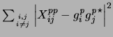 is minimized (see section 7.3).
Normally, Walsh switching (Thompson et al.1986) is used to
eliminate the polarization leakage due to cross-talk between the
signal paths, such that
is minimized (see section 7.3).
Normally, Walsh switching (Thompson et al.1986) is used to
eliminate the polarization leakage due to cross-talk between the
signal paths, such that
![]() . However,
. However,
![]() s can also be finite due to mechanical imperfections in the feed
or the cross-polar primary beam, which cannot be eliminated by Walsh
switching.
s can also be finite due to mechanical imperfections in the feed
or the cross-polar primary beam, which cannot be eliminated by Walsh
switching.
In the case of significant antenna based polarization leakage
(compared to
![]() ), the second term in
Equation 7.3 involving
), the second term in
Equation 7.3 involving
![]() s will combine with the closure
noise
s will combine with the closure
noise
![]() . The polarization leakage therefore manifests
itself as increased closure errors (see Section 7.5 for
a geometric explanation on the Poincaré sphere). This has also been
pointed out by Rogers (1983) in the context of VLBA
observations. However, as written in Equation 7.3, the
leakages and gains are actually antenna based quantities and can be
solved for, using only the co-polar visibilities.
. The polarization leakage therefore manifests
itself as increased closure errors (see Section 7.5 for
a geometric explanation on the Poincaré sphere). This has also been
pointed out by Rogers (1983) in the context of VLBA
observations. However, as written in Equation 7.3, the
leakages and gains are actually antenna based quantities and can be
solved for, using only the co-polar visibilities.
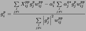
In the absence of any polarization leakage, ![]() s can be estimated by
minimizing
s can be estimated by
minimizing
with respect to ![]() s, where
s, where
![]() ,
,
![]() being the variance on the measurement of
being the variance on the measurement of
![]() .
.
In Equation 7.2, if
![]() accurately represents the
source structure,
accurately represents the
source structure,
![]() will have no source structure dependent
terms and is purely a product of two antenna dependent complex gains.
For a resolved source,
will have no source structure dependent
terms and is purely a product of two antenna dependent complex gains.
For a resolved source,
![]() can be estimated from the image of
the source.
can be estimated from the image of
the source.
Evaluating
![]() and equating it to
zero10.2(see Appendix D), we get
and equating it to
zero10.2(see Appendix D), we get
This can also be derived by equating the partial derivatives of ![]() with respect to real and imaginary parts of
with respect to real and imaginary parts of
![]() .
.
Since the antenna dependent complex gains also appear on the
right-hand side of Equation 7.5, it has to be solved iteratively
starting with some initial guess for ![]() s or initializing them all
to 1. Equation 7.5 can be written in the iterative form as:
s or initializing them all
to 1. Equation 7.5 can be written in the iterative form as:
where ![]() is the iteration number and
is the iteration number and
![]() . Convergence
would be defined by the constraint
. Convergence
would be defined by the constraint
![]() (the change in
(the change in ![]() from one iteration to another) where,
from one iteration to another) where, ![]() is
the tolerance limit and must be related to the average value of
is
the tolerance limit and must be related to the average value of
![]() . Equation 7.6 forms the central engine for
the classical antsol algorithm used for primary calibration of the
visibilities and in self-calibration for imaging purposes. This algorithm
was suggested by Thompson & D'Addario (1982).
. Equation 7.6 forms the central engine for
the classical antsol algorithm used for primary calibration of the
visibilities and in self-calibration for imaging purposes. This algorithm
was suggested by Thompson & D'Addario (1982).
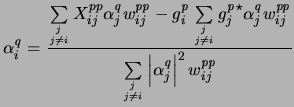
In the presence of significant polarization leakage, Equation 7.3 can be used to re-write Equation 7.4 as
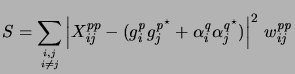 |
(10.7) |
In this form, ![]() is an estimator for the true closure
noise
is an estimator for the true closure
noise
![]() rather than the artificially increased closure
noise (
rather than the artificially increased closure
noise (
![]() ) due to the presence of
polarization leakage.
) due to the presence of
polarization leakage.
Equating the partial derivatives
![]() ,
,
![]() to
zero, we get
to
zero, we get
These non-linear equations can also be iteratively solved.
Equation 7.3, which expresses the observed visibilities on a
point source unpolarized calibrator in terms of the gains and leakage
coefficients of the antennas, would take the same form if written in
an arbitrary orthogonal basis. It is clear that the ![]() 's and the
's and the
![]() 's will change when we change the basis, so this means that
the equations cannot have a unique solution. This situation is
familiar from ordinary self-calibration, when only relative phases of
antennas are determinate, with one antenna acting as an arbitrary
reference. For observations of unpolarized sources, we can similarly
say that any feed can be chosen as a reference polarization, with zero
leakage, and other feeds have gains and leakages in the basis defined
by this reference. Other conventions may be more convenient, as
discussed in Section 7.6 which discusses degeneracy
in detail.
's will change when we change the basis, so this means that
the equations cannot have a unique solution. This situation is
familiar from ordinary self-calibration, when only relative phases of
antennas are determinate, with one antenna acting as an arbitrary
reference. For observations of unpolarized sources, we can similarly
say that any feed can be chosen as a reference polarization, with zero
leakage, and other feeds have gains and leakages in the basis defined
by this reference. Other conventions may be more convenient, as
discussed in Section 7.6 which discusses degeneracy
in detail.
We simulated visibilities with varying fraction of polarization
leakage in the antennas to test the algorithm as follows. The antenna
based signal and leakage were constructed as ![]() and
and
![]() where
where ![]() and
and ![]() were drawn from
the same gaussian random population. The visibility from two antennas
were drawn from
the same gaussian random population. The visibility from two antennas
![]() and
and ![]() was then constructed as
was then constructed as
![]() for
for
![]() . This is
equivalent to a visibility of an unpolarized point source of unit
strength with a complex antenna based gain
. This is
equivalent to a visibility of an unpolarized point source of unit
strength with a complex antenna based gain ![]() and leakage
and leakage
![]() of strength proportional to
of strength proportional to ![]() . Equation 7.6 was
then used to compute
. Equation 7.6 was
then used to compute ![]() and residual
and residual ![]() computed as
computed as
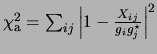 . The computed values of
![]() were then used to
compute improved estimates for
were then used to
compute improved estimates for
![]() by simultaneously solving for
by simultaneously solving for
![]() and
and
![]() using the iterative forms of Equations 7.8 and
7.9. The derived values of
using the iterative forms of Equations 7.8 and
7.9. The derived values of
![]() and
and
![]() matched the true
values to within the tolerance limit. A new
matched the true
values to within the tolerance limit. A new ![]() was computed as
was computed as
 . The values of
![]() and
and
![]() as a function of
as a function of ![]() are
plotted in Fig. 7.1. The two curves become
distinguishable when the leakage is significantly greater than
are
plotted in Fig. 7.1. The two curves become
distinguishable when the leakage is significantly greater than
![]() (for
(for ![]() greater than
greater than ![]() %). After that, the
value of
%). After that, the
value of
![]() is consistently lower than
is consistently lower than
![]() , where the contribution of antenna based leakage
has not been removed. Also notice that
, where the contribution of antenna based leakage
has not been removed. Also notice that
![]() remains
constant while
remains
constant while
![]() quadratically increases as a
function of
quadratically increases as a
function of ![]() . This is due to the fact that antsol treats the
antenna based polarization leakage as closure errors resulting in an
increased
. This is due to the fact that antsol treats the
antenna based polarization leakage as closure errors resulting in an
increased ![]() with increasing fractional leakage.
with increasing fractional leakage.
![\includegraphics[]{Images/leaky_simulations.2.ps}](img1040.png)
|
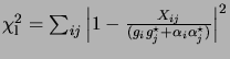
Engineering measurements for polarization isolation at 150 MHz for the
GMRT show significant polarization leakage in the system. We
therefore used leaky antsol to calibrate the data from the Galactic
plane phase calibrator 1830-36 which is known to be less than
![]() polarized at 1.4 GHz. The percentage polarization at 150 MHz
is not known, but it is expected to decrease further and it was taken
to be an unpolarized point source.
polarized at 1.4 GHz. The percentage polarization at 150 MHz
is not known, but it is expected to decrease further and it was taken
to be an unpolarized point source.
Fractional polarization leakage (
![]() ) of up to
100% was measured for most of the antennas, which is consistent with
the estimated leakage measured from system engineering tests. Again,
) of up to
100% was measured for most of the antennas, which is consistent with
the estimated leakage measured from system engineering tests. Again,
![]() and
and
![]() were computed and the
results are shown in Fig. 7.2. The 150-MHz GMRT
band suffers from severe radio frequency interference (RFI). The
sharp rise in the value of
were computed and the
results are shown in Fig. 7.2. The 150-MHz GMRT
band suffers from severe radio frequency interference (RFI). The
sharp rise in the value of
![]() around sample number 10
is due to one such RFI spike. This spike is present in the total
power data from all antennas at this time. On an average, the
around sample number 10
is due to one such RFI spike. This spike is present in the total
power data from all antennas at this time. On an average, the
![]() reduces by
reduces by ![]() when leakage calibration is applied
(
when leakage calibration is applied
(
![]() ). This is consistent with polarization leakage
being a major source of non-closure at this frequency.
). This is consistent with polarization leakage
being a major source of non-closure at this frequency.
![\includegraphics[]{Images/rms.150.1830-36.ps}](img1044.png)
|
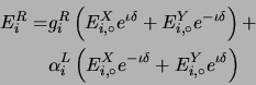
The GMRT L-band feeds are linearly polarized. For the purpose of a VLBI experiment conducted in December 2000, the L-band feed of one of the antennas was converted to a circularly polarized feed. The rest of the L-band feeds were linearly polarized and we took this opportunity to measure correlations between the circularly polarized antenna with other linearly polarized antennas using the source 3C147. Two scans of approximately one hour long observations were done using the single side band GMRT correlator. This correlator computes only co-polar visibilities. With this configuration of feeds, visibilities between the circularly polarized antenna and all other linearly polarized antennas corresponds to correlation between the nominal X- and R-polarizations, labeled by RX, were recorded in the first scan. The polarization of the circularly polarized antenna was then flipped for the second scan to record the correlation between the nominal X- and L-polarization states, labeled by LX.
The VLA Calibrator Manual10.3 lists the percentage polarization
(
 ) for 3C147 at L-band
![]() . The cross-polar terms in Equation 7.2, which are
assumed to be zero, will therefore contribute an error of the order of
. The cross-polar terms in Equation 7.2, which are
assumed to be zero, will therefore contribute an error of the order of
![]() . These cross-polar terms will be, however, multiplied by
gains of type
. These cross-polar terms will be, however, multiplied by
gains of type
![]() . Since
. Since
![]() and
and
![]() are both
assumed to be uncorrelated between antennas, this error will manifest
as random noise in Equation 7.3. Within the limits of other
sources of errors, the source 3C147 can therefore be considered
to be a completely unpolarized source.
are both
assumed to be uncorrelated between antennas, this error will manifest
as random noise in Equation 7.3. Within the limits of other
sources of errors, the source 3C147 can therefore be considered
to be a completely unpolarized source.
![\includegraphics[]{Images/pcs.bnw.epsi}](img1055.png)
|
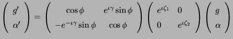
The response of an ideal circularly polarized antenna to unpolarized
incident radiation can be expressed as a superposition of two linear
polarization states as
![]() where, the superscripts
where, the superscripts ![]() ,
, ![]() and
and ![]() denote the right circular and the two linear polarization
states respectively.
denote the right circular and the two linear polarization
states respectively.
![]() is half the phase difference between the two linear
polarization states and is equal to
is half the phase difference between the two linear
polarization states and is equal to ![]() for right-circular
polarization and
for right-circular
polarization and ![]() for left-circular polarization. Writing the
general Equation 7.1 for right-circularly polarized antenna
as
for left-circular polarization. Writing the
general Equation 7.1 for right-circularly polarized antenna
as
![]() and
substituting for
and
substituting for
![]() and
and
![]() we get
we get
 |
(10.10) |
Equation 7.3 for the case of correlation between a circularly polarized and a linearly polarized antenna, with polarization leakage in both the antennas, can be written as
 |
(10.11) |
where
![]() and
and
![]() . The leaky antsol solutions for the
circularly polarized antenna in this case will correspond to
. The leaky antsol solutions for the
circularly polarized antenna in this case will correspond to
![]() and
and
![]() .
.
Let
![]() (
(
![]() for the circularly polarized antenna). Then, the amplitude of
for the circularly polarized antenna). Then, the amplitude of ![]() is a measure of the fractional polarization leakage in the antenna
while the phase of
is a measure of the fractional polarization leakage in the antenna
while the phase of ![]() gives the phase difference between the signal
from one of the feeds and the leaked signal from the other feed. For
an ideal circularly polarized antenna,
gives the phase difference between the signal
from one of the feeds and the leaked signal from the other feed. For
an ideal circularly polarized antenna,
![]() . A plot of
the real and imaginary parts of this quantity for all antennas should
therefore clearly show
. A plot of
the real and imaginary parts of this quantity for all antennas should
therefore clearly show ![]() for the circularly polarized antenna with
an amplitude of 1 and at an angle of
for the circularly polarized antenna with
an amplitude of 1 and at an angle of ![]() with respect to the
nominal X-axis.
with respect to the
nominal X-axis.
The real and imaginary parts of ![]() for all antennas from this
experiment are shown in Fig. 7.3. The solutions were
computed for every integration cycle of
for all antennas from this
experiment are shown in Fig. 7.3. The solutions were
computed for every integration cycle of ![]() sec and the points
on this plot represent the tip of phasor
sec and the points
on this plot represent the tip of phasor ![]() . The collection of
points near the origin are for all the linearly polarized antennas
while the collection of two sets of points away from the origin,
approximately an angle of
. The collection of
points near the origin are for all the linearly polarized antennas
while the collection of two sets of points away from the origin,
approximately an angle of ![]() from each other, are for the
circularly polarized antenna. The solutions found by leaky antsol match the expected results quite well. This therefore constitutes a
reasonably controlled test with real data showing that the solutions
indeed provide information about the polarization leakage in the
system.
from each other, are for the
circularly polarized antenna. The solutions found by leaky antsol match the expected results quite well. This therefore constitutes a
reasonably controlled test with real data showing that the solutions
indeed provide information about the polarization leakage in the
system.
This experiment however provides much more information about the
polarization properties of the antenna feeds used. The collection of
points in the first quadrant denoted by open circles are the values of
![]() derived from the correlation between the nominal
right-circularly polarized signal and the linearly polarized signals
along the nominal X-axis from all other antennas. Points in the third
quadrant are similarly derived using the left-circular signals. The
set of points denoted by triangles in the second and fourth quadrant
are derived using correlations of right- and left-circularly polarized
signals with the linearly polarized signals along the nominal Y-axis
from all other antennas.
derived from the correlation between the nominal
right-circularly polarized signal and the linearly polarized signals
along the nominal X-axis from all other antennas. Points in the third
quadrant are similarly derived using the left-circular signals. The
set of points denoted by triangles in the second and fourth quadrant
are derived using correlations of right- and left-circularly polarized
signals with the linearly polarized signals along the nominal Y-axis
from all other antennas.
A larger spread in the solutions using the left-circularly polarized
signals indicates that the closure noise (from other unknown sources)
in these signals is higher. The fact that the amplitude of ![]() derived using the right-circularly polarized signals is
derived using the right-circularly polarized signals is
![]() indicates that the nominal circularly polarized feed is in fact
elliptically polarized with this axial ratio. The spread of
indicates that the nominal circularly polarized feed is in fact
elliptically polarized with this axial ratio. The spread of ![]() about the origin is indicative of polarization leakage at the
level of few percent in the linearly polarized antennas as well. The
leakage in one of the linearly polarized antennas is significantly
larger (
about the origin is indicative of polarization leakage at the
level of few percent in the linearly polarized antennas as well. The
leakage in one of the linearly polarized antennas is significantly
larger (
![]() ). Since this kind of data is routinely taken on
primary calibrators during GMRT observations for synthesis imaging,
leaky antsol provides a useful diagnostic of system health,
polarization performance and numbers needed to correct the data in
high accuracy work.
). Since this kind of data is routinely taken on
primary calibrators during GMRT observations for synthesis imaging,
leaky antsol provides a useful diagnostic of system health,
polarization performance and numbers needed to correct the data in
high accuracy work.
The following test was also carried out to check that the closure phase on a triangle involving the circular feed was indeed mainly due to polarization effects. The three baselines making up this triangle were flagged as bad baselines from the input data and a new solution found for the gains and leakages of all antennas. This solution predicted the same closure phase (to within errors) as actually observed.
In this section we use right- and left-circular polarization states as
the basis. A general elliptically polarized state can be written as a
superposition of two states represented by the vector
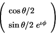 . Clearly,
![]() corresponds to linear
polarization and
corresponds to linear
polarization and
![]() to elliptical polarization (see
Fig. 7.4). Increasing
to elliptical polarization (see
Fig. 7.4). Increasing ![]() by
by ![]() rotates
the direction of the linear state or the major axis of the ellipse by
rotates
the direction of the linear state or the major axis of the ellipse by
![]() . We can chose the phase of the basis so that
. We can chose the phase of the basis so that ![]() corresponding to linear polarization along the x-axis. The Poincaré
sphere representation of the state of polarization maps the general
elliptic state to the point (
corresponding to linear polarization along the x-axis. The Poincaré
sphere representation of the state of polarization maps the general
elliptic state to the point (
![]() ) on the sphere. The properties of this representation are
reviewed by Ramachandran & Ramaseshan (1961). We are concerned here
with one remarkable property, discovered by
Pancharatnam (1956); Pancharatnam (1975). Whenever there is
constructive interference between two sources of radiation, it is
natural to regard them as in phase. A remarkable property of this
simple definition manifests itself when we consider 3 sources of
radiation of different polarization - that if a source A is in phase
with B and B in phase with C, C in general need not be in phase with
A. The phase difference between A and C is known in the optics
literature as the geometric or Pancharatanam phase (see also
Ramaseshan & Nityananda (1986); Berry (1987)). We show that this naturally
occurs in radio interferometry of an unpolarized source with three
antennas of different polarizations.
) on the sphere. The properties of this representation are
reviewed by Ramachandran & Ramaseshan (1961). We are concerned here
with one remarkable property, discovered by
Pancharatnam (1956); Pancharatnam (1975). Whenever there is
constructive interference between two sources of radiation, it is
natural to regard them as in phase. A remarkable property of this
simple definition manifests itself when we consider 3 sources of
radiation of different polarization - that if a source A is in phase
with B and B in phase with C, C in general need not be in phase with
A. The phase difference between A and C is known in the optics
literature as the geometric or Pancharatanam phase (see also
Ramaseshan & Nityananda (1986); Berry (1987)). We show that this naturally
occurs in radio interferometry of an unpolarized source with three
antennas of different polarizations.
![\includegraphics[]{Images/poincare_sphere.ps}](img1085.png)
|
Let the polarization states of the three antennas be represented by
 ,
,
 , and
, and
 in a
circular basis. Denoting the vector
in a
circular basis. Denoting the vector
 by
by ![]() , one clearly see that the
visibility on the 1-2 baseline is proportional to
, one clearly see that the
visibility on the 1-2 baseline is proportional to
![]() . Hence the closure phase around a triangle made by antennas
1, 2, and 3 is the phase of the complex number (also called the triple
product)
. Hence the closure phase around a triangle made by antennas
1, 2, and 3 is the phase of the complex number (also called the triple
product)
![]() . In the quantum mechanical literature, this type of quantity
goes by the name of Bargmann's invariant and its connection to the
geometric phase was made clear by Samuel & Bhandari (1988). With
some work, one can give a general proof that the closure phase (phase
of
. In the quantum mechanical literature, this type of quantity
goes by the name of Bargmann's invariant and its connection to the
geometric phase was made clear by Samuel & Bhandari (1988). With
some work, one can give a general proof that the closure phase (phase
of ![]() ) is equal to half the solid angle subtended at the centre
of the Poincaré sphere by the points represented by
) is equal to half the solid angle subtended at the centre
of the Poincaré sphere by the points represented by ![]() ,
,
![]() , and
, and ![]() on the surface of the sphere. For the case
where the polarization state of the three antennas are same, this
phase is zero in general. However, when the polarization states of
the antennas are different, this phase is non-zero.
on the surface of the sphere. For the case
where the polarization state of the three antennas are same, this
phase is zero in general. However, when the polarization states of
the antennas are different, this phase is non-zero.
The well known result that an arbitrary polarization state can be
represented as a superposition of two orthogonal polarization states
translates to representing any point on the Poincaré sphere by the
superposition of two diametrically opposite states on a great circle
passing through that point. For example, circular polarization can be
expressed by two linear polarizations, each with intensity
![]() . In the context of the present work, the nominally
circularly polarized antenna maps to a point away from the equator on
the Poincaré sphere (it would be exactly on the pole if it is purely
circular) while the rest of the antennas map close to the equator
(they would be exactly on the equator if they are purely linear and
map to a single point if they were also identical). The visibility
phase due to the extra baseline based term in Equation 7.3 due
to polarization mis-match is a consequence of the Pancharatanam phase
mentioned above. This phase, on a triangle involving the circularly
polarized antenna, will be close to the angle between the two linear
antennas. For example, if
. In the context of the present work, the nominally
circularly polarized antenna maps to a point away from the equator on
the Poincaré sphere (it would be exactly on the pole if it is purely
circular) while the rest of the antennas map close to the equator
(they would be exactly on the equator if they are purely linear and
map to a single point if they were also identical). The visibility
phase due to the extra baseline based term in Equation 7.3 due
to polarization mis-match is a consequence of the Pancharatanam phase
mentioned above. This phase, on a triangle involving the circularly
polarized antenna, will be close to the angle between the two linear
antennas. For example, if
 ,
,
 , and
, and
 , the phase of
 ![]() will be
will be
![]() . This picture can be depicted by plotting the real and
imaginary parts of
. This picture can be depicted by plotting the real and
imaginary parts of
![]() , which is done in
Fig. 7.3. The circularly polarized antenna can be
clearly located in this figure as the set of point away from the
origin while the linearly polarized antennas as the set of points
close to the origin. The collection of points located away but almost
symmetrically about the origin represents the nominal right- and
left-circularly polarized feeds. Points on the equator, but
significantly away from the origin represents an imperfect linearly
polarized antenna. Note that the average closure phase between the
nominally linear antennas is close to zero, which defines the mean
reference frame in Fig. 7.3.
, which is done in
Fig. 7.3. The circularly polarized antenna can be
clearly located in this figure as the set of point away from the
origin while the linearly polarized antennas as the set of points
close to the origin. The collection of points located away but almost
symmetrically about the origin represents the nominal right- and
left-circularly polarized feeds. Points on the equator, but
significantly away from the origin represents an imperfect linearly
polarized antenna. Note that the average closure phase between the
nominally linear antennas is close to zero, which defines the mean
reference frame in Fig. 7.3.
We discuss the non-uniqueness of the solutions of
Equation 7.3, and possible convenient conventions for choosing
a specific solution. One obvious degeneracy is that multiplication of
all the ![]() 's by one common phase factor independent of antenna,
and all the
's by one common phase factor independent of antenna,
and all the ![]() 's, by another, in general different, common factor,
does not affect the right hand side of Equation 7.3. Also, the
equation was written in a specific basis, say right and left
circular. But it would have had the same form when using any other
orthogonal pair as basis. Hence we are free to apply this change of
basis to one solution to get another solution of
Equation 7.3. Under such a change, the coefficients transform
according to
's, by another, in general different, common factor,
does not affect the right hand side of Equation 7.3. Also, the
equation was written in a specific basis, say right and left
circular. But it would have had the same form when using any other
orthogonal pair as basis. Hence we are free to apply this change of
basis to one solution to get another solution of
Equation 7.3. Under such a change, the coefficients transform
according to
 |
(10.12) |
It is easy to verify that under this change,
![]() . Clearly, since
. Clearly, since ![]() is unchanged
by these transformations, an iterative algorithm will simply pick one
member of the set of possible solutions, determined by the initial
conditions. Having found one such, one could apply a suitable
transformation to obtain a solution satisfying some desired
condition. For example, if one has nominally linear feeds, one might
impose the statistical condition that there is some mean linear basis
with respect to which the leakage coefficients will be as small as
possible. Such a condition has the advantage that a perfect set of
feeds is not described in a roundabout way as a set of leaky feeds
with identical coefficients, simply because the basis chosen was
different. Carrying out the minimization of
is unchanged
by these transformations, an iterative algorithm will simply pick one
member of the set of possible solutions, determined by the initial
conditions. Having found one such, one could apply a suitable
transformation to obtain a solution satisfying some desired
condition. For example, if one has nominally linear feeds, one might
impose the statistical condition that there is some mean linear basis
with respect to which the leakage coefficients will be as small as
possible. Such a condition has the advantage that a perfect set of
feeds is not described in a roundabout way as a set of leaky feeds
with identical coefficients, simply because the basis chosen was
different. Carrying out the minimization of
![]() by the method of Lagrange multipliers, subject to a constant
by the method of Lagrange multipliers, subject to a constant ![]() ,
we obtain the condition that
,
we obtain the condition that
![]() . This solution can
be interpreted as requiring the leakage coefficients to be orthogonal
to the gains, and is reasonable when we think about the opposite kind
of situation, when the leakages are "parallel" to the gains,
i.e. identical apart from a multiplicative constant. In such a case,
we would obviously change the basis to make the new leakage zero. If
we have a solution which does not satisfy this orthogonality
condition, we can bring it about in two steps. First, choose an
overall phase for the
. This solution can
be interpreted as requiring the leakage coefficients to be orthogonal
to the gains, and is reasonable when we think about the opposite kind
of situation, when the leakages are "parallel" to the gains,
i.e. identical apart from a multiplicative constant. In such a case,
we would obviously change the basis to make the new leakage zero. If
we have a solution which does not satisfy this orthogonality
condition, we can bring it about in two steps. First, choose an
overall phase for the ![]() 's so that
's so that
![]() is
real. Then, carry out a rotation in the
is
real. Then, carry out a rotation in the
![]() plane by an angle
plane by an angle
![]() satisfying
satisfying
![]() . This rotation has been so chosen
that it makes the leakage "orthogonal" to the gains, in the sense
required above. Even after this is done, we still have the freedom to
define the phase zero independently for the two orthogonal
states. This is because we are only dealing with unpolarized
sources. Of course, if we had a linearly polarized calibrator, the
relative phase of right and left circular signals would not be
arbitrary.
. This rotation has been so chosen
that it makes the leakage "orthogonal" to the gains, in the sense
required above. Even after this is done, we still have the freedom to
define the phase zero independently for the two orthogonal
states. This is because we are only dealing with unpolarized
sources. Of course, if we had a linearly polarized calibrator, the
relative phase of right and left circular signals would not be
arbitrary.
A more geometric view of this degeneracy is obtained when we think in terms of the Poincaré sphere representation of the states of polarization of all the feeds. The cross correlation between the outputs of two feeds, both of which receive unpolarized radiation, has a magnitude equal to the cosine of half the angle between the representative points on the sphere. Measurements of all such cross correlations with unpolarized radiation fixes the relative geometry of the points on the sphere, while leaving a two parameter degeneracy corresponding to overall rigid rotations of the sphere. This degeneracy can be lifted by the measurement of one polarized source at many parallactic angles.
Finally, we note that for the purpose of correcting the observations of unpolarized sources for the effects of non-identical feed polarization, the degeneracy is unimportant, because the correction factor is precisely the right hand side of Equation 7.3 which is unaffected by all the transformations we have discussed.
Rogers (1983) pointed out that non ideal feed polarizations of the individual antennas of a radio interferometer can result into closure errors in the co-polar visibilities. In this chapter we described and demonstrated a method to measure the polarization leakage of individual antennas using the nominally co-polar visibilities for an unpolarized calibrator. This method can therefore be used as a useful tool for studying the polarization purity of the antennas of radio interferometers from the observations of unpolarized calibrators. However, since only unpolarized calibrators are used, the actual solution for the leakage parameters is subject to a degeneracy. This degeneracy does not affect the correction of the visibilities and can be used to remove the closure errors due to polarization leakage. Massi et al. (1997) have shown that such polarization leakage induced closure errors in the data from the EVN is the dominant effect of instrumental polarization. For the EVN, this effect can be seen as a reduction in the dynamic range of the images. Our method can be used for such data to remove these closure errors for unpolarized sources.
The general elliptic state of the polarization of radiation can be represented by a point on the Poincaré sphere. The phase difference between three coherent sources of radiation but with different states of polarization goes by the name of Pancharatanam or geometric phase in the optics literature. We interpret the co-polar visibilities with polarization leakages on the Poincaré sphere and show that the polarization induced closure phase errors in radio interferometers is same as the Pancharatanam phase of optics. The antenna based leakages also map to points on the Poincaré sphere and the ambiguity in the solution can be understood as a rigid rotation of the Poincaré sphere, which leaves the leakage solutions unchanged relative to each other.

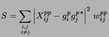

![$\displaystyle {g_i^{\it p}}^{,n} = {g_i^{\it p}}^{,n-1} + \lambda\left[{g_i^{\i...
...i}} \left\vert{g_j^{\it p}}^{,n-1}\right\vert^2 w_{ij}^{{\it p}{\it p}}}\right]$](img1017.png)