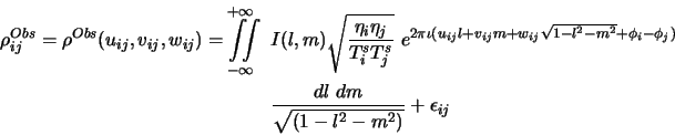
In practice, however, the antenna based amplitude
(
![]() ) and phase (
) and phase (![]() ) are potentially time
varying quantities. This could be due to changes in the ionosphere,
temperature variations, ground pick up, antenna blockage, noise pick
up by various electronic components, background temperature, etc.
Treating the quantities under the square root in the above equation as
the antenna dependent amplitude gains, these can be written as complex
gains
) are potentially time
varying quantities. This could be due to changes in the ionosphere,
temperature variations, ground pick up, antenna blockage, noise pick
up by various electronic components, background temperature, etc.
Treating the quantities under the square root in the above equation as
the antenna dependent amplitude gains, these can be written as complex
gains
![]() where
where
![]() . For
an unresolved source at the phase tracking center, variations in this
amplitude will be indistinguishable from a variations in the ratio of
. For
an unresolved source at the phase tracking center, variations in this
amplitude will be indistinguishable from a variations in the ratio of
![]() and
and ![]() .
.
In terms of ![]() s, we can write Equation D.1 as
s, we can write Equation D.1 as
| (15.2) |
 |
(15.3) |
For an unresolved source at the phase tracking center, all terms in
the exponent of
![]() are exactly zero.
are exactly zero.
![]() in this case would be proportional to the flux density of the source.
in this case would be proportional to the flux density of the source.
Assuming that the antenna dependent complex gains are independent,
with a gaussian probability density function (this implies that the
real and imaginary parts are independently gaussian random processes),
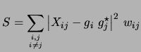
one can estimate ![]() s by minimizing, with respect to
s by minimizing, with respect to ![]() s, the
function
s, the
function ![]() given by
given by
 |
(15.4) |
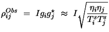
Dividing the above equation by
![]() (the source model,
which is presumed to be known - it is trivially known for an
unresolved source), and writing
(the source model,
which is presumed to be known - it is trivially known for an
unresolved source), and writing
![]() , we get
, we get
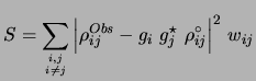
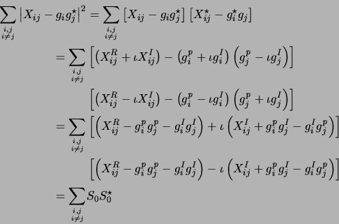
Expanding Equation D.5, we get
![$\displaystyle S=\sum_{{i,j} \atop {i \ne j}}\left[ \left\vert X_{ij}\right\vert...
...X_{ij} - g_i g_j^\star X_{ij}^\star + g_i g_i^\star g_j g_j^\star\right] w_{ij}$](img1140.png) |
(15.6) |
![$\displaystyle {\partial S \over \partial g_i^\star} = \sum_{j \atop {j \ne i}}\left[-g_j X_{ij} w_{ij} +g_i g_j g_j^\star w_{ij}\right] = 0$](img1143.png) |
(15.7) |
This can also be derived by equating the partial derivatives of ![]() with respect to real and imaginary parts of
with respect to real and imaginary parts of ![]() as shown in
Section D.3.
as shown in
Section D.3.
Since the antenna dependent complex gains also appear on the
right-hand side of Equation D.8, it has to be solved
iteratively starting with some initial guess for ![]() s or
initializing them all to 1.
s or
initializing them all to 1.
Equation D.8 can be written in the iterative form as:
(the change in ![]() from one iteration to another) where
from one iteration to another) where ![]() is
the tolerance limit.
is
the tolerance limit.
![]() is a product of two complex numbers, namely
is a product of two complex numbers, namely ![]() and
and
![]() , which we wish to determine.
, which we wish to determine. ![]() is itself derived
from the measured quantity
is itself derived
from the measured quantity
![]() . Numerically speaking, each
term in the summation of the numerator of Equation D.8
will involve
. Numerically speaking, each
term in the summation of the numerator of Equation D.8
will involve ![]() (via
(via ![]() ) and the multiplication of
) and the multiplication of ![]() with
with
![]() would give
would give ![]() an effective weight of
an effective weight of
![]() . Since the denominator is the sum of this
effective weight, the right-hand side of Equation D.8 can
be interpreted as the weighted average of
. Since the denominator is the sum of this
effective weight, the right-hand side of Equation D.8 can
be interpreted as the weighted average of ![]() over all correlations
with antenna
over all correlations
with antenna ![]() .
.
In the very first iteration, when ![]() , the normalization would
be incorrect since the numeric value of
, the normalization would
be incorrect since the numeric value of ![]() , as it appears inside
, as it appears inside
![]() would be different from that used in the denominator of
Equation D.8. However, as the estimates of
would be different from that used in the denominator of
Equation D.8. However, as the estimates of ![]() s improve
with iterations, the equation would progressively approach a true
weighted average equation. The speed of convergence will depend upon
the value of
s improve
with iterations, the equation would progressively approach a true
weighted average equation. The speed of convergence will depend upon
the value of ![]() and the convergence would be defined by the
constraint in Equation D.10. In the ideal case
when the true value of all
and the convergence would be defined by the
constraint in Equation D.10. In the ideal case
when the true value of all ![]() s is known, right hand side of
Equation D.8 also reduces of
s is known, right hand side of
Equation D.8 also reduces of ![]() .
.
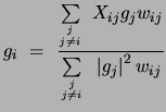
Estimating ![]() for an antenna, by averaging over the measurements
from all baselines in which it participates (for a unresolved source)
makes sense since for an N element array,
for an antenna, by averaging over the measurements
from all baselines in which it participates (for a unresolved source)
makes sense since for an N element array, ![]() would be present in
N-1 measurements (all the
would be present in
N-1 measurements (all the
![]() ) and
the best estimate of
) and
the best estimate of ![]() would be the weighted average of all these
measurements. Proper weight for
would be the weighted average of all these
measurements. Proper weight for ![]() , buried in each of the products
, buried in each of the products
![]() , can be found heuristically as follows.
, can be found heuristically as follows. ![]() , estimated
from the measurements of a given baseline, must obviously be weighted
by the signal-to-noise ratio on that baseline. This is
, estimated
from the measurements of a given baseline, must obviously be weighted
by the signal-to-noise ratio on that baseline. This is ![]() in
the above equations. It must also be weighted by the amplitude gain
of the other antenna making the baseline, namely
in
the above equations. It must also be weighted by the amplitude gain
of the other antenna making the baseline, namely ![]() , to account for
variation in antenna sensitivities and
, to account for
variation in antenna sensitivities and ![]() . The total weight for
. The total weight for
![]() would then be
would then be
![]() , the sum of which
appears in the denominator of Equation D.8. Knowing that
ideally
, the sum of which
appears in the denominator of Equation D.8. Knowing that
ideally
![]() , each of the
, each of the
![]() must be multiplied by
must be multiplied by
![]() (to apply
the the above mentioned weights to
(to apply
the the above mentioned weights to ![]() ), before being summed for all
values of
), before being summed for all
values of ![]() and normalized by the sum of weights to form the
weighted average of
and normalized by the sum of weights to form the
weighted average of ![]() . One thus arrives at
Equation D.8 using these heuristic arguments.
. One thus arrives at
Equation D.8 using these heuristic arguments.
 |
(15.11) |
 |
(15.12) |
All contributions to
![]() , which cannot be factored into
antenna dependent gains, will result in the reduction of
, which cannot be factored into
antenna dependent gains, will result in the reduction of
![]() .
. ![]() remaining constant, this will be
indistinguishable from an increase in the effective system
temperature. Since majority of later processing of interferometry
data for mapping (primary calibration, bandpass calibration, SelfCal,
etc.) is done by treating the visibility as a product of two antenna
based numbers, this is the effective system temperature which will
determine the noise in the final map (though, as a final step in the
mapping process, baseline based calibration can possibly improve the
noise in the map).
remaining constant, this will be
indistinguishable from an increase in the effective system
temperature. Since majority of later processing of interferometry
data for mapping (primary calibration, bandpass calibration, SelfCal,
etc.) is done by treating the visibility as a product of two antenna
based numbers, this is the effective system temperature which will
determine the noise in the final map (though, as a final step in the
mapping process, baseline based calibration can possibly improve the
noise in the map).
In the normal case of no significant baseline based terms
(
![]() ) in
) in ![]() , the system temperature as measured by
the above method will be equivalent to any other determination of
, the system temperature as measured by
the above method will be equivalent to any other determination of
![]() .
.
![]() can also be determined by recording interferometric data for a
strong point source with and without an independent noise source of
known temperature at each antenna. In this case
can also be determined by recording interferometric data for a
strong point source with and without an independent noise source of
known temperature at each antenna. In this case
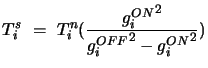 |
(15.13) |
Expanding Equation D.5, ignoring ![]() s and writing it
in terms of real and imaginary parts we get
s and writing it
in terms of real and imaginary parts we get
| (15.15) |
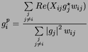
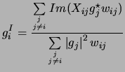
![$\displaystyle {\partial S \over \partial g_i^I}=-2\sum\limits_{j \atop {j \ne i}}\left[Im(X_{ij}g_j^\star) - \left\vert g_j\right\vert^2 g_i^I\right] w_{ij}$](img1177.png) |
(15.19) |
![$\displaystyle g_i^n = g_i^{n-1} + \alpha\left[g_i^{n-1}-{\sum\limits_{j \atop {...
...sum\limits_{j \atop {j \ne i}} \left\vert g_j^{n-1}\right\vert^2 w_{ij}}\right]$](img1145.png)
![\begin{displaymath}\begin{split}{\partial S \over \partial {g_i^{\it p}}}=&\sum\...
...I}^2 - {g_i^{\it p}} {{g_j^{\it p}}}^2\right]w_{ij} \end{split}\end{displaymath}](img1173.png)
![$\displaystyle {\partial S \over \partial {g_i^{\it p}}}= -2\sum\limits_{j \atop...
...t[Re(X_{ij}g_j^\star ) - \left\vert g_j\right\vert^2 {g_i^{\it p}}\right]w_{ij}$](img1174.png)