![\includegraphics[]{XYCoordsys.eps}](img224.png)
|
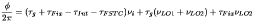
An aperture synthesis telescope, like the GMRT, consists of a number
of antennas located on the ground and the resolution of such a
telescope is proportional to the maximum projected separation between
the antennas. The locations of the antennas are usually specified in
the Earth-centred ![]() co-ordinate system. The Earth centred
co-ordinate system. The Earth centred ![]() frame is related to the
frame is related to the ![]() location of the antennas on the ground
by
location of the antennas on the ground
by
However, for the purpose of imaging, only the relative separation
between the antennas is important. This separation between the
antennas is usually referred to as the baseline and is measured
in units of the wavelength ![]() of the incident radiation. For
the purpose of the theory of synthesis imaging, the antenna positions
are specified in the so called
of the incident radiation. For
the purpose of the theory of synthesis imaging, the antenna positions
are specified in the so called ![]() frame. The geometric
relationship between this
frame. The geometric
relationship between this ![]() frame and the
frame and the ![]() frame is shown in
Fig. 2.1 and the co-ordinate transformation is given by
frame is shown in
Fig. 2.1 and the co-ordinate transformation is given by
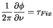
The geometric relation between the observing plane represented by the
![]() -plane and the sky plane represented by the
-plane and the sky plane represented by the ![]() -plane is shown in
Fig. 2.2. The
-plane is shown in
Fig. 2.2. The ![]() -plane in the sky is parallel to the plane
in which measurements are made (the
-plane in the sky is parallel to the plane
in which measurements are made (the ![]() -plane) and the separation
between them is denoted by
-plane) and the separation
between them is denoted by ![]() . The
. The ![]() -axis points towards the
origin of the
-axis points towards the
origin of the ![]() frame given by (
frame given by (![]() ,
,![]() ) and is parallel to
the
) and is parallel to
the ![]() -axis. The treatment of the theory of synthesis imaging given
below follows that of Thompson et al. (1986) and
Clark (1999).
-axis. The treatment of the theory of synthesis imaging given
below follows that of Thompson et al. (1986) and
Clark (1999).
Let
![]() represent the electric field produced by
an infinitesimal element in the sky in the direction
represent the electric field produced by
an infinitesimal element in the sky in the direction ![]() at
point
at
point ![]() in the
in the ![]() frame (Fig. 2.2). The total
electric field
frame (Fig. 2.2). The total
electric field
![]() measured at this point will be an
integral of the signals from all the radiation elements and is given
by
measured at this point will be an
integral of the signals from all the radiation elements and is given
by
![\includegraphics[scale=0.6]{2DGeom.2.ps}](img242.png)
|
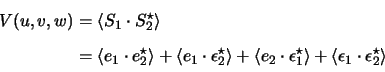
The source coherence function, defined as
The mutual coherence function, measured at two points
![]() and
and ![]() on the observing plane is defined as
on the observing plane is defined as
where
![]() is the relative delay
between the signals measured at the points
is the relative delay
between the signals measured at the points ![]() and
and ![]() respectively.
respectively.
In the above equation, the dependence on ![]() and
and ![]() is implicitly via
is implicitly via ![]() . For a plane wavefront from a direction
. For a plane wavefront from a direction
![]() in the sky,
in the sky,
![]() where
where
![]() is the vector separating the two antennas. It is
therefore clear that
is the vector separating the two antennas. It is
therefore clear that ![]() depends only on the relative separation
between the antenna positions given by
depends only on the relative separation
between the antenna positions given by ![]() and
and ![]() and
can be written as
and
can be written as
| (5.9) |
In the limit of the plane wave front approximation, the denominator in
Equation 2.8 can be adequately represented by
![]() and
and
![]() . The phase of the
mutual coherence function in Equation 2.7,
for a spatially incoherent source, therefore, depends only on the
relative separation between the points of measurement in the far field
of the radiation.
. The phase of the
mutual coherence function in Equation 2.7,
for a spatially incoherent source, therefore, depends only on the
relative separation between the points of measurement in the far field
of the radiation.
Let
![]() represent the unit vector along the
represent the unit vector along the ![]() -axis
pointing towards (
-axis
pointing towards (![]() ). The components of
). The components of
![]() in
the
in
the ![]() frame will be (0,0,1). The relative delay between the
signals received at the two antennas from a point source in this
direction will be
frame will be (0,0,1). The relative delay between the
signals received at the two antennas from a point source in this
direction will be
![]() . Treating
. Treating
![]() as the reference direction
towards the origin of the source co-ordinate system, the instantaneous
phase of
as the reference direction
towards the origin of the source co-ordinate system, the instantaneous
phase of
![]() can be measured with respect to this
direction, without losing any information about the sky brightness
distribution. This can be done by rotating the phase of
can be measured with respect to this
direction, without losing any information about the sky brightness
distribution. This can be done by rotating the phase of ![]() by
by
![]() . The point in the sky in the direction
. The point in the sky in the direction
![]() is referred to as the phase centre and
is referred to as the phase centre and ![]() is referred to as the geometrical delay. The Phase centre
direction defines the origin of the source co-ordinate system. Since
is referred to as the geometrical delay. The Phase centre
direction defines the origin of the source co-ordinate system. Since
![]() is an arbitrary vector, the phase centre can be
chosen at any convenient point in the sky. Usually, this is
coincident with the antenna pointing centre.
is an arbitrary vector, the phase centre can be
chosen at any convenient point in the sky. Usually, this is
coincident with the antenna pointing centre.
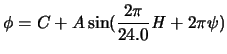
The visibility phase for a point source at the phase centre,
after correcting for the geometrical phase is equal to zero.
With this correction, the visibility is said to be `phased' for the
phase centre. An interferometer phased for this reference
direction will remain phased for all points on the surface of a sphere
of unit radius passing through the point (![]() ), centred at
(
), centred at
(![]() ) and described by the equation
) and described by the equation
![]() . Under
ideal conditions (i.e., with no other source of phase errors), any
residual phase would be due to the relative separation between the
phase centre and a source of emission located on such a sphere.
In that sense, the visibility phase from a `phased' interferometer
provides information about the distribution of the sky brightness,
relative to the phase centre. Moving one of the antennas to the
origin of the
. Under
ideal conditions (i.e., with no other source of phase errors), any
residual phase would be due to the relative separation between the
phase centre and a source of emission located on such a sphere.
In that sense, the visibility phase from a `phased' interferometer
provides information about the distribution of the sky brightness,
relative to the phase centre. Moving one of the antennas to the
origin of the ![]() frame, the (
frame, the (
![]() ) co-ordinates
are just the co-ordinates of the other antenna and the subscript
`
) co-ordinates
are just the co-ordinates of the other antenna and the subscript
`![]() ' can be dropped from Equation 2.10.
' can be dropped from Equation 2.10.
The length of time for which a signal remains coherent is given by the
inverse of the bandwidth
![]() . After correcting for the geometrical delay, the relative delay between the signals is
. After correcting for the geometrical delay, the relative delay between the signals is
![]() . Replacing
. Replacing ![]() by
by ![]() in
Equation 2.8 corresponds to the geometrical delay
corrected version of this equation. If
in
Equation 2.8 corresponds to the geometrical delay
corrected version of this equation. If
![]() ,
two versions of a time series displaced with respect to each other in
time by
,
two versions of a time series displaced with respect to each other in
time by ![]() will remain coherent. In the limit of the validity
of the assumption that
will remain coherent. In the limit of the validity
of the assumption that
![]() ,
,
![]() in
Equation 2.8 can be replaced by
in
Equation 2.8 can be replaced by
![]() .
This is the same as the source auto-correlation function at zero lag,
.
This is the same as the source auto-correlation function at zero lag,
![]() (Equation 2.6) and is equal to the
two dimensional source surface brightness, denoted by
(Equation 2.6) and is equal to the
two dimensional source surface brightness, denoted by ![]()
Therefore, under the approximation that:
using the relation between ![]() in Equation 2.10 and the above
mentioned phase rotation, Equation 2.8 can be
re-written as
in Equation 2.10 and the above
mentioned phase rotation, Equation 2.8 can be
re-written as
The integrals in the above equation are over the entire sky (limits of
the integral from ![]() to
to ![]() ). However, the antenna primary beam
limits the part of the sky from which the antenna can receive
radiation to
). However, the antenna primary beam
limits the part of the sky from which the antenna can receive
radiation to
![]() , where
, where ![]() is the diameter of a circular
aperture. Assuming that the response close to the centre of the
primary beam is
is the diameter of a circular
aperture. Assuming that the response close to the centre of the
primary beam is ![]() , with an additional approximation that the
field of view is small (
, with an additional approximation that the
field of view is small (
![]() ),
Equation 2.11 can be written as
),
Equation 2.11 can be written as
The source surface brightness ![]() is described in the
is described in the ![]() -plane
while
-plane
while ![]() and
and ![]() are the equivalent conjugate variables in Fourier
space.
are the equivalent conjugate variables in Fourier
space. ![]() and
and ![]() can therefore be interpreted as the spatial
frequencies and the visibility function as the spatial frequency
spectrum of the source surface brightness distribution. Synthesis
radio telescopes like the GMRT measure the visibility function
at several points in the
can therefore be interpreted as the spatial
frequencies and the visibility function as the spatial frequency
spectrum of the source surface brightness distribution. Synthesis
radio telescopes like the GMRT measure the visibility function
at several points in the ![]() frame using an array of
frame using an array of ![]() antennas
which instantaneously produce
antennas
which instantaneously produce ![]() pairs of interferometers.
Due to the rotation of the earth, the projected separations between
the antennas change as the antennas track a source in the sky. Over
time, each antenna pair therefore measures the visibility at several
points in the
pairs of interferometers.
Due to the rotation of the earth, the projected separations between
the antennas change as the antennas track a source in the sky. Over
time, each antenna pair therefore measures the visibility at several
points in the ![]() frame. As a result, over time, the array of
antennas partially covers the
frame. As a result, over time, the array of
antennas partially covers the ![]() volume, up to a maximum projected
antenna separation of
volume, up to a maximum projected
antenna separation of ![]() corresponding to a spatial resolution
of
corresponding to a spatial resolution
of ![]() . Also, an interferometric array does not measure
. Also, an interferometric array does not measure ![]() for baselines smaller than a minimum value. Just as the maximum
baseline length for which
for baselines smaller than a minimum value. Just as the maximum
baseline length for which ![]() is measured corresponds to the highest
spatial resolution the telescope can provide, the smallest baseline
for which
is measured corresponds to the highest
spatial resolution the telescope can provide, the smallest baseline
for which ![]() is measured corresponds to largest angular scale that
can be represented reliably in the final image. Hence, an
interferometric observation will be insensitive to scales larger than
is measured corresponds to largest angular scale that
can be represented reliably in the final image. Hence, an
interferometric observation will be insensitive to scales larger than
![]() ; this problem of missing short spacing measurements is
referred to as the problem of ``missing short spacing''. When imaging
extended objects in the sky, like the ones imaged for this
dissertation, the shortest spacing for which a reliable measurement
exist has for reaching implications - missing short spacings result
in missing extended emission in the image.
; this problem of missing short spacing measurements is
referred to as the problem of ``missing short spacing''. When imaging
extended objects in the sky, like the ones imaged for this
dissertation, the shortest spacing for which a reliable measurement
exist has for reaching implications - missing short spacings result
in missing extended emission in the image.
If
![]() is completely sampled, at least at the Nyquist rate,
it can be inverse Fourier transformed to recover the source brightness
distribution
is completely sampled, at least at the Nyquist rate,
it can be inverse Fourier transformed to recover the source brightness
distribution ![]() . With a finite number of antennas located at
discrete locations on the ground, the visibility function is
sampled at a discreet set of points. The observed visibility can,
therefore, be thought of as the true visibility, multiplied by the sampling
function given by
. With a finite number of antennas located at
discrete locations on the ground, the visibility function is
sampled at a discreet set of points. The observed visibility can,
therefore, be thought of as the true visibility, multiplied by the sampling
function given by
| (5.13) |
The approximation that
![]() breaks down at low
frequencies and Equation 2.11 accurately described
the measured visibility function. However, this is not a
Fourier transform relation. Techniques used to recover
breaks down at low
frequencies and Equation 2.11 accurately described
the measured visibility function. However, this is not a
Fourier transform relation. Techniques used to recover ![]() in such
cases are described in Chapter 4.
in such
cases are described in Chapter 4.
![\includegraphics[]{2Ant.ps}](img312.png)
|
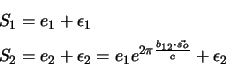
In practice, ![]() is measured by a number of two element
interferometers, one of which is shown in Fig. 2.3. The
signal from antenna 1 lags behind the signal from the antenna
2 by a phase equal to
is measured by a number of two element
interferometers, one of which is shown in Fig. 2.3. The
signal from antenna 1 lags behind the signal from the antenna
2 by a phase equal to
![]() where
where ![]() is the reference unit vector mentioned in the
previous section. Under the plane wave approximation, the signals
from the two antennas can be written as
is the reference unit vector mentioned in the
previous section. Under the plane wave approximation, the signals
from the two antennas can be written as
 |
(5.14) |
 |
(5.15) |
The response of the interferometer to a point source of flux density
![]() , located at the phase centre (
, located at the phase centre (![]() ) is therefore
) is therefore
Antennas receive radiation from a finite part of the sky, defined by
the antenna primary beam. For an extended source, within the antenna
primary beam, ![]() will be an integral over the source (integral
over
will be an integral over the source (integral
over ![]() and
and ![]() ;Equation 2.12) and can be thought of as a
superposition of plane waves from the individual infinitesimal
elements constituting the extended source given by
Equation 2.17.
;Equation 2.12) and can be thought of as a
superposition of plane waves from the individual infinitesimal
elements constituting the extended source given by
Equation 2.17.
As the interferometer tracks the source in the sky, the projected
separation and hence the geometrical delay changes with time.
![]() changes slowly going from
changes slowly going from
![]() to
to
![]() when the antennas track a source from rise to set over several hours.
when the antennas track a source from rise to set over several hours.
![]() depends on the declination of the source and the
minimum elevation limits of the antennas. Over short intervals of
time,
depends on the declination of the source and the
minimum elevation limits of the antennas. Over short intervals of
time, ![]() changes almost linearly with time. The interferometer
response to a point source (the real and imaginary parts) therefore
varies quasi-sinusoidally over short periods of time with a frequency
proportional to the separation between the antennas. This
quasi-sinusoidal variation of the interferometer output, due to the
changing geometrical delay, is referred to as the fringe
pattern. The amplitude of this fringe pattern is directly
proportional to the power emitted by the source in the sky. The phase
of these fringes also changes sinusoidally with time with a period of
24 hours. The phase of this fringe pattern due to the geometrical delay however carries no astronomically useful
information about the sky (it only carries information about the
direction in the sky being tracked). In practice therefore, the geometrical delay is continuously compensated by introducing a time
variable compensating delay
changes almost linearly with time. The interferometer
response to a point source (the real and imaginary parts) therefore
varies quasi-sinusoidally over short periods of time with a frequency
proportional to the separation between the antennas. This
quasi-sinusoidal variation of the interferometer output, due to the
changing geometrical delay, is referred to as the fringe
pattern. The amplitude of this fringe pattern is directly
proportional to the power emitted by the source in the sky. The phase
of these fringes also changes sinusoidally with time with a period of
24 hours. The phase of this fringe pattern due to the geometrical delay however carries no astronomically useful
information about the sky (it only carries information about the
direction in the sky being tracked). In practice therefore, the geometrical delay is continuously compensated by introducing a time
variable compensating delay ![]() in the signal from one of the
antennas. This operations is referred to as delay tracking.
The radio-frequency (RF) signals from the antenna feeds, centred at a
frequency
in the signal from one of the
antennas. This operations is referred to as delay tracking.
The radio-frequency (RF) signals from the antenna feeds, centred at a
frequency
![]() , are converted to an intermediate frequency
band centred at
, are converted to an intermediate frequency
band centred at
![]() to be transported to the correlator
(in the case of GMRT, over optical fiber cables). The path length for
the signals from the antenna to the correlator introduces a time
invariant fixed delay
to be transported to the correlator
(in the case of GMRT, over optical fiber cables). The path length for
the signals from the antenna to the correlator introduces a time
invariant fixed delay
![]() suffered by the signals at
suffered by the signals at
![]() . The compensating delay
. The compensating delay ![]() must therefore compensate
for
must therefore compensate
for
![]() as well.
as well.
For the GMRT, the compensating delay
![]() is
applied to the signals at baseband frequencies in the correlator.
However, the signals suffer the delays
is
applied to the signals at baseband frequencies in the correlator.
However, the signals suffer the delays ![]() and
and
![]() at the
RF and IF frequencies respectively. Delay compensation at the
baseband therefore leaves a residual phase given by
at the
RF and IF frequencies respectively. Delay compensation at the
baseband therefore leaves a residual phase given by
Effectively, the phase of the visibilities is rotated by
![]() , equivalent to the residual delay due to the differences in the
RF, IF and base band frequencies. The phase of the visibility for a
point source located at the phase centre is thus reduced to zero at
all times. This final rotation of the fringe phase is referred to as
fringe stopping or fringe rotation.
, equivalent to the residual delay due to the differences in the
RF, IF and base band frequencies. The phase of the visibility for a
point source located at the phase centre is thus reduced to zero at
all times. This final rotation of the fringe phase is referred to as
fringe stopping or fringe rotation.
Note that the total phase applied to the visibilities via delay
tracking and fringe rotation is equal to ![]() and this
effectively phases the interferometer for a point in the sky (the
phase centre). Application of this total phase is achieved in the
GMRT correlator in two stages, as explained in
Section 2.5.2.
and this
effectively phases the interferometer for a point in the sky (the
phase centre). Application of this total phase is achieved in the
GMRT correlator in two stages, as explained in
Section 2.5.2.
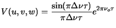
The response of the interferometer is integrated over the signal
bandwidth as seen by the multiplier in the correlator. If ![]() represents the voltage response of the antennas as seen by the
multiplier, the effect of a finite bandwidth is to modulate the output
of the interferometer by the Fourier transform of
represents the voltage response of the antennas as seen by the
multiplier, the effect of a finite bandwidth is to modulate the output
of the interferometer by the Fourier transform of ![]() . If the
receiver has a flat response for a range of frequencies
. If the
receiver has a flat response for a range of frequencies
![]() , the output
, the output ![]() , for a source of unit flux density, will
be given by
, for a source of unit flux density, will
be given by
 |
(5.19) |
![]() is the relative antenna separation along the
is the relative antenna separation along the ![]() -axis. As is
clear from Equation 2.2, the geometrical delay involves the
measurement of the relative (
-axis. As is
clear from Equation 2.2, the geometrical delay involves the
measurement of the relative (![]() ) co-ordinates of different
antennas. It is therefore important to measure the relative antenna
co-ordinates as well as the fixed delays for phasing the array
(reducing the fringe phase to zero for the phase centre). The
procedure used for measuring the relative antenna co-ordinates
(referred to as baseline calibration) and fixed delays
(referred to as fixed delay calibration) for the GMRT is
described in Sections 2.6.1
and 2.6.2 respectively.
) co-ordinates of different
antennas. It is therefore important to measure the relative antenna
co-ordinates as well as the fixed delays for phasing the array
(reducing the fringe phase to zero for the phase centre). The
procedure used for measuring the relative antenna co-ordinates
(referred to as baseline calibration) and fixed delays
(referred to as fixed delay calibration) for the GMRT is
described in Sections 2.6.1
and 2.6.2 respectively.
As mentioned earlier, ![]() is measured for several values of
is measured for several values of
![]() and
and ![]() by tracking the source in the sky for several hours,
during which the projected baseline of a single interferometer changes
with time. In practice, a number of antennas are used and the output
of all the
by tracking the source in the sky for several hours,
during which the projected baseline of a single interferometer changes
with time. In practice, a number of antennas are used and the output
of all the ![]() interferometer pairs made by an array of
interferometer pairs made by an array of ![]() antennas provide instantaneous measurements at several values of
antennas provide instantaneous measurements at several values of ![]() and
and ![]() . The instantaneous set of points measured in the
. The instantaneous set of points measured in the ![]() frame
by an array of antennas is referred to as the snapshot
uv-coverage. As the array tracks a source in the sky, each
interferometer generates a track in the uv-plane, dramatically
increasing the uv-coverage of the array. The set of
frame
by an array of antennas is referred to as the snapshot
uv-coverage. As the array tracks a source in the sky, each
interferometer generates a track in the uv-plane, dramatically
increasing the uv-coverage of the array. The set of ![]() points, measured by an array of antennas over several hours of source
tracking, is referred to as the full synthesis uv-coverage. The
shape and density of the uv-coverage of the array determines the
telescope transfer function and the geometry of the array is usually
optimized to maximize the uv-coverage (Mathur1969). The
configuration of the 30-antenna GMRT array and resulting uv-coverage are described in Section 2.2.
points, measured by an array of antennas over several hours of source
tracking, is referred to as the full synthesis uv-coverage. The
shape and density of the uv-coverage of the array determines the
telescope transfer function and the geometry of the array is usually
optimized to maximize the uv-coverage (Mathur1969). The
configuration of the 30-antenna GMRT array and resulting uv-coverage are described in Section 2.2.
The GMRT antennas are fully steerable parabolic dishes each of 45m
diameter each with an Alt-azimuth mount. A turret at the prime focus
of the antenna is supported by a quadripod and holds a sealed metallic
cube which houses the broadband low noise amplifier (LNA), RF filters,
the polarizer and the RF switch for swapping the polarization channels
for each RF band (see Section 2.3). The feeds for 150,
327, 233/610, and 1420 MHz are mounted on the four faces of the turret
which can be rotated to bring the desired feed in focus using the feed positioning system (FPS). The feed bandwidths and the range of
frequencies covered by the various feeds are listed in
Table 2.1. The feed bandwidths correspond to a
Standing wave ratio of ![]() . The 233-MHz feed has the smallest
bandwidth while the cross-polar characteristic of the 150-MHz feed is
the worst. The measured cross-polar power at 327 and 610 MHz bands is
. The 233-MHz feed has the smallest
bandwidth while the cross-polar characteristic of the 150-MHz feed is
the worst. The measured cross-polar power at 327 and 610 MHz bands is
![]() and
and ![]() dB respectively while that for the 150-MHz
feed is
dB respectively while that for the 150-MHz
feed is ![]() dB. The value away from the centre of the
radiation pattern is
dB. The value away from the centre of the
radiation pattern is ![]() dB for 327 and 610 MHz bands while
that for the 150-MHz feed is
dB for 327 and 610 MHz bands while
that for the 150-MHz feed is ![]() dB (see Sankar (2000)
for more details). Since the GMRT is predominantly a low frequency
instrument, the reflecting surface of the antennas is a light weight
wire mesh. The wire mesh is held in place by a network of steel
ropes, creating patches of flat surfaces which approximate a parabola.
This design is referred to as the Stretched Mesh Attached to Rope
Trusses design or the SMART design (Swarup et al.1991). Three sizes of wire
mesh are used, going from smallest sized mesh (10 mm) in the inner
region of the parabola to the largest size (20 mm) towards the edge to
produce a tapered illumination pattern which reduces the side-lobe
levels of the antenna radiation pattern. Mesh of different sizes each
covers one third of the total surface area. The reflecting surface
for each antenna was measured by theodolite, to determine the surface
accuracy compared to an ideal parabola. An RMS deviation of 8, 9 and
14 mm from an ideal parabola was measured for the three regions of the
surface (Sankar2000).
dB (see Sankar (2000)
for more details). Since the GMRT is predominantly a low frequency
instrument, the reflecting surface of the antennas is a light weight
wire mesh. The wire mesh is held in place by a network of steel
ropes, creating patches of flat surfaces which approximate a parabola.
This design is referred to as the Stretched Mesh Attached to Rope
Trusses design or the SMART design (Swarup et al.1991). Three sizes of wire
mesh are used, going from smallest sized mesh (10 mm) in the inner
region of the parabola to the largest size (20 mm) towards the edge to
produce a tapered illumination pattern which reduces the side-lobe
levels of the antenna radiation pattern. Mesh of different sizes each
covers one third of the total surface area. The reflecting surface
for each antenna was measured by theodolite, to determine the surface
accuracy compared to an ideal parabola. An RMS deviation of 8, 9 and
14 mm from an ideal parabola was measured for the three regions of the
surface (Sankar2000).
![\includegraphics[]{Ant_Full.eps}](img356.png) |
| Nominal Centre Freq. | Feed Bandwidth | Freq. Range | Reliable Range |
| (MHz) | (MHz) | (MHz) | (MHz) |
| 150 | 130 | ||
| 233 | 12 | ||
| 327 | 138 | ||
| 610 | 127 | ||
| 1420 | 580 |
![\includegraphics[scale=0.8]{20_full.eps}](img368.png) ![\includegraphics[scale=0.8]{m20_full.eps}](img369.png)
![\includegraphics[scale=0.8]{40_full.eps}](img370.png) ![\includegraphics[scale=0.8]{m40_full.eps}](img371.png) |
![\includegraphics[scale=0.8]{20_csq.eps}](img376.png) ![\includegraphics[scale=0.8]{m20_csq.eps}](img377.png)
![\includegraphics[scale=0.8]{40_csq.eps}](img378.png) ![\includegraphics[scale=0.8]{m40_csq.eps}](img379.png) |
The GMRT is composed of 30 such antennas. The antennas are located in
a roughly `Y' shaped geometry (Mathur1969), as shown in
Fig. 2.4. Fourteen antennas are located randomly in a
region of size ![]() km
km![]() km, referred to as the Central Square
(see Fig. 2.5). These antennas provide the short
spacing coverage of the uv-plane, which is essential for mapping large
scale structures. The rest of the antennas are located in
km, referred to as the Central Square
(see Fig. 2.5). These antennas provide the short
spacing coverage of the uv-plane, which is essential for mapping large
scale structures. The rest of the antennas are located in ![]() km
long Western-, Eastern-, and Southern-arms. The Eastern- and
Southern-arms each have 5 antennas, roughly along a straight line,
while the Western-arm has 6 antennas. This arrangement of antennas
was designed to maximize the telescope sensitivity to large scale
emission as well as to provide high resolution. The shortest spacing
of
km
long Western-, Eastern-, and Southern-arms. The Eastern- and
Southern-arms each have 5 antennas, roughly along a straight line,
while the Western-arm has 6 antennas. This arrangement of antennas
was designed to maximize the telescope sensitivity to large scale
emission as well as to provide high resolution. The shortest spacing
of ![]() m in the Central Square is provided by the antennas C05, C06 and C09
while the largest spacing of
m in the Central Square is provided by the antennas C05, C06 and C09
while the largest spacing of ![]() km is provided by the arm
antennas. The Central Square antennas together provide a uv-coverage up to
1 km. The uv-coverage for a full
km is provided by the arm
antennas. The Central Square antennas together provide a uv-coverage up to
1 km. The uv-coverage for a full ![]() synthesis observation using
the full array is shown in Fig. 2.6. The
uv-coverage due to Central Square antennas alone, for a full
synthesis observation using
the full array is shown in Fig. 2.6. The
uv-coverage due to Central Square antennas alone, for a full ![]() synthesis at
a few declinations is shown in Fig. 2.7.
synthesis at
a few declinations is shown in Fig. 2.7.
A detailed description and analysis of the analog signal flow for the GMRT has been described elsewhere (Praveen Kumar2000; Praveen Kumar & Srinivas1996). This section briefly describes the aspects of the GMRT analog receivers which are relevant from the point of view of astronomical observations.
The GMRT operates at the 150, 233, 327, 610 and L-band extending from
![]() MHz. The L-band is split into four sub-bands centred at
1060, 1170, 1280 and 1390 MHz with a bandwidth of 120 MHz while the
bandwidth at other bands is
MHz. The L-band is split into four sub-bands centred at
1060, 1170, 1280 and 1390 MHz with a bandwidth of 120 MHz while the
bandwidth at other bands is ![]() MHz. Fig. 2.8
shows a simplified schematic diagram, with the major components of
MHz. Fig. 2.8
shows a simplified schematic diagram, with the major components of
![\includegraphics[scale=0.8]{GMRT_RX.PS}](img385.png) |
The RF band is first converted to an IF band centred at 70 MHz using
what is referred to as the First LO (First Local Oscillator).
Here, bandwidths of 5.5, 16 or the full RF bandwidths can be selected.
The two IF signals corresponding to the two polarizations are then
converted to 130 and 175 MHz with a maximum bandwidth of 32 MHz using
the Second LO. These signals are then transported over optical
fibers to the Central Electronics Building (CEB). Variable
attenuators in the range of ![]() dB, which can be varied in steps of
2 dB are available separately for the two IF signals. An automatic
level controller (ALC) at the output of the IF can be bypassed if
required (e.g. for observations requiring measurement of variations at
high time resolution). At the CEB, the 130- and 175-MHz signals,
recovered from the output of the optical fibers, are fed to the Base
Band system for conversion to base-band signals. These signals are
first converted to 70 MHz band and then split into Upper- and
Lower-Sidebands using the tunable Fourth LO. This LO can
be tuned between
dB, which can be varied in steps of
2 dB are available separately for the two IF signals. An automatic
level controller (ALC) at the output of the IF can be bypassed if
required (e.g. for observations requiring measurement of variations at
high time resolution). At the CEB, the 130- and 175-MHz signals,
recovered from the output of the optical fibers, are fed to the Base
Band system for conversion to base-band signals. These signals are
first converted to 70 MHz band and then split into Upper- and
Lower-Sidebands using the tunable Fourth LO. This LO can
be tuned between ![]() MHz in steps of 100 Hz. At the base band,
bandwidths of the 62.5, 125, 250, 500 KHz or 1, 2, 4, 8, 16 MHz can be
selected. Another ALC is provided at the output of the baseband.
Signal levels are kept at 0 dBm by this ALC before being fed to the
correlator (see Section 2.5). This ALC also can,
however, be bypassed.
MHz in steps of 100 Hz. At the base band,
bandwidths of the 62.5, 125, 250, 500 KHz or 1, 2, 4, 8, 16 MHz can be
selected. Another ALC is provided at the output of the baseband.
Signal levels are kept at 0 dBm by this ALC before being fed to the
correlator (see Section 2.5). This ALC also can,
however, be bypassed.
For the purpose of astronomical observations, settings of the attenuators and the First and Fourth LOs are important. The combination of these two LOs determine the exact RF frequency used for observations.
The output of the individual antennas is a random signal composed of
the signals from the source of interest in the sky, the sky background
emission and the thermal noise generated by the various electronic
components through which the signal flows. The output of the antennas
and the receiver is usually expressed in terms of the temperature of a
blackbody which will emit equivalent power. The system
temperature (![]() ) of an antenna at a particular frequency, is
equivalent to the total power from the antenna when it points towards
a blank sky. The power received by an antenna due to the celestial
source alone is represented by the antenna temperature (
) of an antenna at a particular frequency, is
equivalent to the total power from the antenna when it points towards
a blank sky. The power received by an antenna due to the celestial
source alone is represented by the antenna temperature (![]() ).
).
The normalized visibility amplitude from antennas 1 and 2 is given by
 |
(5.20) |
These and other astronomically relevant parameters of the GMRT are listed in Table 2.25.1. Fifth column is listed the angular resolution for both Central Square and full array.
The prototype 4 and 8 antenna correlator, all of the initial design and most of the implementation of the final 30 antenna single sideband correlator currently in use and which was used for the observations for this dissertation were designed and built by the team consisting of C.R.Subramanya, A.Dutta, V.M.Tatke, A.Dikshit, R.K.Malik, U.Puranik, M.Burse and others. Further development for the second sideband correlator and maintenance is now done by Y.Gupta, M.Burse, S.Sirothia, C.P.Kanade, K.H.Dahimiwal, I.Halagalli and others, with contributions from A.Roshi. This section describes aspects of the GMRT correlator relevant from the point of view of astronomical observations. A more detailed description of the current correlator hardware design is given by Tatke (1998). The correlator control and data acquisition software for potentially multiple sub-array mode of operation was designed and implemented by R.K.Singh and C.R.Subrahmanya. A detailed description of the current correlator control and data acquisition software is given by Singh (2000). The sub-array mode of operation is described by Chengalur (2000).
The GMRT back-end for interferometric observations is an FX-type
digital correlator. The block diagram in Fig. 2.9
shows the various stages of the correlator. The first stage of this
correlator consists of a set of four samplers per antenna - one for
each of the two IFs per side-band of the antenna. Each antenna
produces two IFs which can carry either the two orthogonal
polarization signals or the same polarization from two different RF
bands (as in the case of ![]() MHz dual frequency feed). The
analog to digital converter (ADC) of the samplers converts the input
analog signal to 8-bit unsigned numbers. These 8-bit samples are
converted to 6-bit unsigned numbers before being fed to the next stage
of the correlator, referred to as the Delay and Data Preparation
Cards, or the Delay/DPC system. These samples are further
converted to 4-bit signed numbers in the Delay/DPC system (see
the section on Samplers below), before being fed to the next stage of
the correlator. This conversion from 8-bit to 4-bit samples is
required since the VLBA FFT chips used in the correlator work with
4-bit signed numbers. Part of the compensating delay equivalent
to integral units of correlator clock is applied in the Delay/DPC stage. Any residual delay (corresponding to a fraction of
the correlator clock) is applied as a phase ramp across the band,
after the signals have been Fourier transformed (see
Section 2.5.2). The Delay/DPC stage is
followed by the Fast Fourier Transform or the FFT stage which
performs a 512-point FFT corresponding to 256 point complex spectra
(the other 256 points being the complex conjugate spectra). The
output complex numbers are represented in 4,4,4-bit format
consisting of two 4-bit numbers for the mantissa of the real and
imaginary parts and a common 4-bit exponent.
MHz dual frequency feed). The
analog to digital converter (ADC) of the samplers converts the input
analog signal to 8-bit unsigned numbers. These 8-bit samples are
converted to 6-bit unsigned numbers before being fed to the next stage
of the correlator, referred to as the Delay and Data Preparation
Cards, or the Delay/DPC system. These samples are further
converted to 4-bit signed numbers in the Delay/DPC system (see
the section on Samplers below), before being fed to the next stage of
the correlator. This conversion from 8-bit to 4-bit samples is
required since the VLBA FFT chips used in the correlator work with
4-bit signed numbers. Part of the compensating delay equivalent
to integral units of correlator clock is applied in the Delay/DPC stage. Any residual delay (corresponding to a fraction of
the correlator clock) is applied as a phase ramp across the band,
after the signals have been Fourier transformed (see
Section 2.5.2). The Delay/DPC stage is
followed by the Fast Fourier Transform or the FFT stage which
performs a 512-point FFT corresponding to 256 point complex spectra
(the other 256 points being the complex conjugate spectra). The
output complex numbers are represented in 4,4,4-bit format
consisting of two 4-bit numbers for the mantissa of the real and
imaginary parts and a common 4-bit exponent.
![\includegraphics[]{corr_schematic.ps}](img415.png)
|
The correlation between signals from two antennas with the same polarization is referred to as the co-polar visibilities. This correlation is done by multiplying the antenna signals and averaging the result in the correlator. The output of the FFT stage is therefore fed to the Multiplier and Accumulation (MAC) stage of the correlator. Each MAC chip accepts 4 input data streams - 2 IFs from the two antennas. However each MAC can only handle a total of 256 channels per antenna. Therefore, either the number of channels per IF must be reduced from 256 to 128 or, only one IF with all the 256 channels must be fed to the MAC. This reduction of 256 channels for each IF to 128 channels to produce the co-polar visibilities is done by averaging two adjacent frequency channels. However, the GMRT correlator can also be used with a resolution of 256 frequency channels by sacrificing one of the polarization signals from the antennas.
The MAC output format consists of two 15-bit mantissa for real
and imaginary parts and a common 6-bit exponent (this format is
referred to as 15,15,6-bit format). The accumulators in the
MAC stage provide the Short Term Accumulation (STA). Each
STA cycle corresponds to 512 correlator clock cycles, required
for reading the 512 points into the FFT section plus 4 clock
cycles required to set-up the FFT cards before it can perform an FFT.
Thus, each FFT cycle requires 516 correlator clock cycles. The
correlator runs on an effective clock of 32 MHz and the STA accumulates the data for 4096 FFT cycles. Thus, the STA
corresponds to an integration of
![]() ms of time.
(Strictly speaking, the samplers run on a 32 MHz clock. This is the
shortest time resolution that the GMRT correlator can provide. The
Delay/DPC system reads the input data at the rate of 32 MHz but
output data rate is 32.125 MHz. The rest of the correlator operates
at 32.125 MHz to effectively take care of the dead time corresponding
to the 4 clock cycles required for FFT setup).
ms of time.
(Strictly speaking, the samplers run on a 32 MHz clock. This is the
shortest time resolution that the GMRT correlator can provide. The
Delay/DPC system reads the input data at the rate of 32 MHz but
output data rate is 32.125 MHz. The rest of the correlator operates
at 32.125 MHz to effectively take care of the dead time corresponding
to the 4 clock cycles required for FFT setup).
The data rates corresponding to a STA time interval is large
(8 MBytes/sec) and difficult to sustain for any data recording system.
The STA data therefore needs to be integrated further to reduce
the data rate by accumulating in the Long Term Accumulation
(LTA) stage of the correlator. This stage has not yet been
implemented in the hardware and therefore, the STA stage has
been set to integrate for 8192 FFT cycles corresponding to a minimum
integration time of ![]() ms. This brings down the data rates to
4 MBytes/sec and the data is further integrated in the software for an
integration time than can be set by the user to produce the final LTA data. The output of the STA stage is the final product of
the correlator and is produced in the form of three data streams from
the three MAC racks per sideband.
ms. This brings down the data rates to
4 MBytes/sec and the data is further integrated in the software for an
integration time than can be set by the user to produce the final LTA data. The output of the STA stage is the final product of
the correlator and is produced in the form of three data streams from
the three MAC racks per sideband.
All the three MAC output streams are fed to the Data Acquisition System (DAS), via a 16-bit bus. The DAS consists of a dual CPU PC running under the GNU/Linux Operating System (OS) with a data acquisition card on its PCI bus. The STA data from all MACs is acquired on this card at the rate of 4 MBytes/sec consisting of all the 256 channels (256 frequency channels with only one polarization, or 128 channels with both polarizations). The software device driver (which runs in the kernel space of the OS) and the supporting program (running in the user space of the OS) convert the input complex numbers from the correlator representation to the IEEE floating point representation. The software LTA is done at this stage for a time interval set by the user and the data rate further reduced. Through a series of network software, this data is transfered to another machine over the fast Ethernet to be recorded on the disk in what is referred to as the LTA-format (Singh (2000)). The last stage in the chain of software also provide facilities for further integration in time and frequency and for defining sub-arrays, etc. (the usage of the sub-array mode of the software is described by Chengalur (2000)).
The analog-to-digital converter (ADC) used in the GMRT samplers is an
8-bit flash ADC (Tatke1998). The input to these samplers is
the band limited gaussian random noise from the antennas, converted to
base-band (BB) (corresponding to a frequency range of 0 to 16 MHz).
The output power of the baseband system is proportional to the antenna
temperature which is a function of the sky temperature. The sky
temperature, can vary by as much as a factor of ![]() between the
Galactic plane and away from it. However, the samplers are designed
to sample a fixed range of input signal. The BB output signals are
therefore maintained at 0 dbm by the Automatic Level Controller (ALC)
before being fed to the samplers. This corresponds to a peak-to-peak
variation of
between the
Galactic plane and away from it. However, the samplers are designed
to sample a fixed range of input signal. The BB output signals are
therefore maintained at 0 dbm by the Automatic Level Controller (ALC)
before being fed to the samplers. This corresponds to a peak-to-peak
variation of ![]() V spanning the input random signal up to the six
sigma level. In order to preserve the statistical properties of the
input, the
V spanning the input random signal up to the six
sigma level. In order to preserve the statistical properties of the
input, the ![]() comparator voltage levels (in the ADC) must be
optimally set such that the samplers neither saturate when the input
voltage deviates by six sigma from the mean, nor sample the weaker
signals too coarsely (corresponding to much smaller deviations from
the mean). As of now, the
comparator voltage levels (in the ADC) must be
optimally set such that the samplers neither saturate when the input
voltage deviates by six sigma from the mean, nor sample the weaker
signals too coarsely (corresponding to much smaller deviations from
the mean). As of now, the ![]() voltage levels corresponding to 8-bit
sampling are uniformly distributed across this range of voltage,
corresponding to a voltage resolution of 7.8 mV (provisions however
exist for a more sophisticated scheme to distribute the levels across
the range of input signal). However, before being fed to the next
stage of the correlator (namely the Delay/DPC stage), the 8-bits
samples are converted to 6-bit samples by dropping the 2 least
significant bits (LSB) of the samples. Effectively, this corresponds
to
voltage levels corresponding to 8-bit
sampling are uniformly distributed across this range of voltage,
corresponding to a voltage resolution of 7.8 mV (provisions however
exist for a more sophisticated scheme to distribute the levels across
the range of input signal). However, before being fed to the next
stage of the correlator (namely the Delay/DPC stage), the 8-bits
samples are converted to 6-bit samples by dropping the 2 least
significant bits (LSB) of the samples. Effectively, this corresponds
to ![]() levels covering the full range of
levels covering the full range of ![]() V, with a
resolution of 31.25 mV, but which still sample the full range of
the input signal up to six sigma, although at a coarser resolution.
These 6-bit samples are unsigned. Inside the Delay/DPC system these
samples are further converted to 4-bit signed values via a look-up
table. The look-up table is made such that the
V, with a
resolution of 31.25 mV, but which still sample the full range of
the input signal up to six sigma, although at a coarser resolution.
These 6-bit samples are unsigned. Inside the Delay/DPC system these
samples are further converted to 4-bit signed values via a look-up
table. The look-up table is made such that the ![]() levels are again
uniformly distributed for the entire range of the input signal (in
this case, the 6-bit samples). Hence, effectively, the input signal
with 6-bit resolution is further sampled at a coarser resolution of
4-bits without statistically altering the signal.
levels are again
uniformly distributed for the entire range of the input signal (in
this case, the 6-bit samples). Hence, effectively, the input signal
with 6-bit resolution is further sampled at a coarser resolution of
4-bits without statistically altering the signal.
For the purpose of astronomical observations, this entire operation of converting the 8-bit unsigned samples to 4-bit signed samples can be ignored and the GMRT samplers can be treated as an effective 4-bit samplers.
This section describes the mechanisms used in the correlator data acquisition software for deriving accurate time information. This is essentially a description of the work done by Singh (2000).
The input data to the DAS is averaged for a length of time set by the
user to produce the long term accumulated (LTA) data. This interval
is typically set to ![]() sec. The LTA operation is currently done
in the software and may be moved to hardware in future (if required).
sec. The LTA operation is currently done
in the software and may be moved to hardware in future (if required).
As mentioned earlier, a synthesis radio telescope like the GMRT utilizes the earth rotation to synthesize an effective large aperture. To keep the array instantaneously phased, the time varying geometrical delay must be continually compensated. The phasing of the array is therefore a time critical operation requiring accurate time keeping. Accurate time information is also required for proper pointing of the antennas and tracking of an astronomical source. Stamping of astronomical data with accurate time is therefore very important.
Absolute time for the GMRT is kept using the real time clock (RTC) of
the GMRT correlator control computer. This clock is synchronized with
the GPS time using a GPS receiver. The GPS and correlator system
clocks are used to remove any time jumps and/or slow drifts of this
real time computer clock as described below. This time stamping of
the visibility data in the GMRT correlator/data acquisition achieves
an accuracy of
![]() sec.
sec.
The correlator provides a synchronization pulse to the DAS to indicate
the start of each STA cycle via an STA interrupt. This
information is also supplied to the DAS via one of the bits of the
data bus, referred to as the data synchronization bit. The DAS
software uses this information to (1) do a consistency check (2)
determine the start of the STA data in a stream of continuous
data flowing on the data bus from the MAC. The DAS card also receives
an interrupt signal at the start of each minute from the GPS receiver.
The interrupt handler (the software which does time critical
operations when a hardware interrupt is received) for both these
interrupts (STA and GPS interrupts) reads the PC time from the PC RTC
at each interrupt and maintains a list of corresponding PC time
stamps. The list of PC time stamps recorded at each GPS interrupt is
then examined for a constant difference of ![]() minute. A continuous
series is selected such that the time difference between successive
samples is accurate to
minute. A continuous
series is selected such that the time difference between successive
samples is accurate to ![]() sec. This series of PC time stamps is
referred to as a series of ``good'' GPS-interrupted time stamps. This
series is used to set up a linear equation between the GPS time and the
PC time. Since GPS time can be easily converted to the local time
standard (Indian Standard Time or IST), this equation essentially
converts the PC time to accurate IST time. This equation provides a
first order calibration of the PC time, and takes care of any short
glitch in the PC time (which can happen due to variety of reasons
including overloading of the PC bus). Similarly, the PC time is
recorded at each STA interrupt. This list of STA-interrupted PC time stamps is also examined and a continuous
series selected such that the time difference between successive PC
time stamps is equal to one STA cycle, to an accuracy of
sec. This series of PC time stamps is
referred to as a series of ``good'' GPS-interrupted time stamps. This
series is used to set up a linear equation between the GPS time and the
PC time. Since GPS time can be easily converted to the local time
standard (Indian Standard Time or IST), this equation essentially
converts the PC time to accurate IST time. This equation provides a
first order calibration of the PC time, and takes care of any short
glitch in the PC time (which can happen due to variety of reasons
including overloading of the PC bus). Similarly, the PC time is
recorded at each STA interrupt. This list of STA-interrupted PC time stamps is also examined and a continuous
series selected such that the time difference between successive PC
time stamps is equal to one STA cycle, to an accuracy of
![]() sec. This series of ``good'' PC time stamps is used to set up
a linear relation between the PC time and STA time. The PC time
to IST time equation is then used to convert the STA time to IST
time, and is also used to tag each STA data block with a
sequence number.
sec. This series of ``good'' PC time stamps is used to set up
a linear relation between the PC time and STA time. The PC time
to IST time equation is then used to convert the STA time to IST
time, and is also used to tag each STA data block with a
sequence number.
The three sources of timing information to the DAS (1) the STA
interrupts (2) the GPS interrupts, and (3) the data synchronization
bit, all provide time information with respect to the PC RTC. In the
above scheme, on a short time scale, unless all these three sources
produce drifts and/or glitches, time stamping of the data will remain
accurate to ![]() sec. Since all these are independently running
clocks, the probability of all three producing error at the same time
is very low and it has been shown that the above time stamping scheme
is quite robust to short time scale glitches and time drifts.
sec. Since all these are independently running
clocks, the probability of all three producing error at the same time
is very low and it has been shown that the above time stamping scheme
is quite robust to short time scale glitches and time drifts.
To account for slow drifts in the PC time, an attempt is made to set up
a new linear equation between the STA sequence number and PC
time after every 16 STA cycles. The new relation is not
accepted unless it matches with the previous one within ![]() sec.
Similarly, a new relation is set up between GPS and PC time at each GPS
interrupt.
sec.
Similarly, a new relation is set up between GPS and PC time at each GPS
interrupt.
On a longer time scale, an error can occur due to some catastrophic error in either of these sources (e.g. the interrupts not arriving at the PC due to hardware failures). If the DAS software cannot set up the new equations for more than a threshold time interval, it is assumed that an irrecoverable error has occurred rendering the current equations invalid. In such a case, the DAS sets up fresh equations and the data between such an event and the time interval required to set up valid equations is unreliable and is flagged. In practice, however, such events are very infrequent.
However, a slow drift in the PC RTC, with respect to which all three sources of timing information are measured, can produce a drift in the final IST time stamps in the data. Data blocks are expected to arrive at the DAS at a pre-determined constant rate. Data blocks themselves therefore can be effectively used as yet another clock, which is independent of the PC time. Any drift of the PC clock will show up as a consistent shift in the equations between the GPS and PC time and between STA and PC time with respect to the arrival of the data blocks. Hence, any consistent error in the arrival of the data blocks measured with respect to the IST time, derived from the two linear equations, will indicate a drift in the PC time. This fact is used to monitor a slow drift in the PC time over the time scale of setting up new equations.
The PC time is also synchronized to the minute pulse from the GPS.
Errors in the PC RTC less than half a minute can therefore be
corrected and PC clock synchronized to the GPS clock. However if the
PC RTC is in error by more than half a minute, this synchronization
will result into minimum of 1 min in the PC RTC. It is therefore
important to set the PC RTC to within ![]() min of the GPS time.
min of the GPS time.
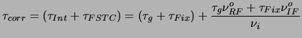
As mentioned earlier, the compensating delay (equal to
![]() ; see Section 2.1.1, page
; see Section 2.1.1, page
![]() ) which needs to be applied to one of the
antennas of an interferometer is applied in the GMRT correlator in two
stages. A delay equivalent to an integral multiple of the correlator
clock (
) which needs to be applied to one of the
antennas of an interferometer is applied in the GMRT correlator in two
stages. A delay equivalent to an integral multiple of the correlator
clock (
![]() ) is applied in the Delay/DPC section of the
correlator. The input data stream is copied into a dual port RAM at
the location given by the write-counter. Data is read simultaneously
from this RAM from the location given by the read-counter. The offset
between the read- and the write-counters for this RAM is maintained
such that the read-counter lags behind the write-counter. Since the
output samples are read with a time delay (equal to the difference
between the counters multiplied by the correlator clock cycle), the
output data stream corresponds to the input data stream with a time
delay. The time delay, however, can only be in multiples of the
correlator clock cycle. The residual delay, corresponding to a
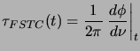
fraction of the correlator clock cycle is applied in the fractional sample time correction or FSTC operation. The
last stage of the FFT butterfly network provides a facility to apply a
channel dependent phase. The frequency channel dependent time
varying, phase corresponding to this residual delay, represented by
) is applied in the Delay/DPC section of the
correlator. The input data stream is copied into a dual port RAM at
the location given by the write-counter. Data is read simultaneously
from this RAM from the location given by the read-counter. The offset
between the read- and the write-counters for this RAM is maintained
such that the read-counter lags behind the write-counter. Since the
output samples are read with a time delay (equal to the difference
between the counters multiplied by the correlator clock cycle), the
output data stream corresponds to the input data stream with a time
delay. The time delay, however, can only be in multiples of the
correlator clock cycle. The residual delay, corresponding to a
fraction of the correlator clock cycle is applied in the fractional sample time correction or FSTC operation. The
last stage of the FFT butterfly network provides a facility to apply a
channel dependent phase. The frequency channel dependent time
varying, phase corresponding to this residual delay, represented by
![]() , is applied as a linear phase gradient across the band
as
, is applied as a linear phase gradient across the band
as
 |
(5.21) |
The output of the FFT stage of the correlator is a set of 256 independent complex numbers. These complex numbers are represented by three 4-bit numbers; one each for the mantissa of real and imaginary parts and one for a common exponent. The complex gains, applicable at the last stage of the FFT butterfly network, are represented by 5 bits each for the real and imaginary parts but has no exponent bit. Thus the channel dependent phase gradient for the FSTC is also limited to a 5-bit representation.
The FFT stage of the correlator performs a real-time Fourier
transform of the input signal effectively splitting the input
bandwidth of
![]() into 128 frequency channels, each of width
into 128 frequency channels, each of width
![]() (the FFT stage of the correlator can be
treated as a set of 128 filter banks). The time series from each of
the 128 frequency channels from an antenna, are then multiplied with
the corresponding channels from all other antennas, before being
integrated in the MAC section of the correlator. The effective
input bandwidth, as seen by the multiplier is therefore
(the FFT stage of the correlator can be
treated as a set of 128 filter banks). The time series from each of
the 128 frequency channels from an antenna, are then multiplied with
the corresponding channels from all other antennas, before being
integrated in the MAC section of the correlator. The effective
input bandwidth, as seen by the multiplier is therefore
![]() . For the GMRT, the maximum value of
. For the GMRT, the maximum value of
![]() is 16 MHz
corresponding to a maximum channel width of
is 16 MHz
corresponding to a maximum channel width of ![]() KHz, giving a fringe washing function of width
KHz, giving a fringe washing function of width
![]() sec. Therefore, for
the GMRT correlator, the residual delay must remain less than a
fraction of this width (typically less then few micro seconds).
sec. Therefore, for
the GMRT correlator, the residual delay must remain less than a
fraction of this width (typically less then few micro seconds).
In the final double sideband correlator, in the continuum, non-polar mode, the correlator can be used to record the two co-polar visibilities (the nominal RR and LL correlations) per antenna with a full bandwidth of 32 MHz (both sidebands). In the current single sideband correlator only one sideband of 16 MHz can be processed. In the full polar mode, which will be available with the dual sideband correlator, the cross polar visibilities (namely RL and LR) cal also be recorded. Since the correlator can handle only 256 channels per antenna at the MAC stage, the cross polar mode can be used with only one of the sidebands with a maximum bandwidth of 16 MHz.
The GMRT correlator naturally produces spectral visibilities with a
maximum of 256 channels across the entire observing band, if only one
polarization is used, or with 128 channels, if both polarizations are
used. For normal continuum observations, the 128 channels across a
16 MHz band provide a channel resolution of ![]() kHz. For
observations where bandwidth smearing is not important (and in the
absence of RFI), these channels can be collapsed on-line to produce
continuum visibilities. At lower frequencies where primary beams are
large, bandwidth smearing can be important for sources away from the
phase centre. Also, at frequencies below
kHz. For
observations where bandwidth smearing is not important (and in the
absence of RFI), these channels can be collapsed on-line to produce
continuum visibilities. At lower frequencies where primary beams are
large, bandwidth smearing can be important for sources away from the
phase centre. Also, at frequencies below ![]() MHz, intermittent RFI
is always a possibility. To reduce bandwidth smearing and to detect
and flag narrow band RFI-contaminated data, all the 128 channels are
usually recorded. Provision for frequency averaging before recording
does however exist and can be used where RFI and bandwidth smearing
problems are not perceived to be serious.
MHz, intermittent RFI
is always a possibility. To reduce bandwidth smearing and to detect
and flag narrow band RFI-contaminated data, all the 128 channels are
usually recorded. Provision for frequency averaging before recording
does however exist and can be used where RFI and bandwidth smearing
problems are not perceived to be serious.
For spectral line observations, channel resolution can be increased by
controlling the sampling rate of the input signal. The sampling rate
can be changed between 32 MHz and 0.125 MHz in steps of two. This
corresponds to an effective bandwidth between 16 MHz and 0.25 MHz with
a frequency resolution between 125 kHz and ![]() kHz
respectively.
kHz
respectively.
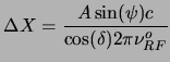
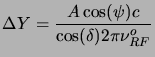
A synthesis radio telescope measures the two-dimensional spatial
frequency spectrum of the source structure. Instantaneous projected
separations between the elements of the interferometer in the uvw-frame determine the spatial frequency being sampled by the
antenna pairs. The projected separation between the antennas, given by
![]() , gives rise to the geometrical delay which needs to be
compensated by delay tracking before the signals are multiplied.
The value of
, gives rise to the geometrical delay which needs to be
compensated by delay tracking before the signals are multiplied.
The value of ![]() is given by
is given by
The radio frequency (RF) signals from the two orthogonal feeds of the antenna are converted to two separate intermediate frequencies (IF) and brought to the Central Electronics building (CEB) for correlation via the optical fiber cables. The fixed delay suffered by the signals from each antenna varies from antenna to antenna since the physical length of the optical fibers to various antennas differ. This fixed delay is largely constant, showing small and slow variations due to changing ground temperature. Since the optical fiber cables are dispersive, any relative fixed delay between antenna pairs results in a time invariant phase ramp across the band in the visibility data. This phase ramp must also be removed or calibrated before averaging the channels to produce the continuum visibilities or before being used for imaging.
The following two sections describe the methodology used and results of baseline and fixed delay calibration.
Historically, the GMRT antenna positions were first determined using theodolite measurements. These were refined using P-band observations following the procedure laid down by Bhatnagar & Rao (1996). Later, dual frequency GPS measurements (Kulkarni1997) were done to independently determine the antenna co-ordinates.
The GPS measurements provided the antenna co-ordinates relative to the
reference GPS antenna, to a quoted accuracy of ![]() cm. However,
monitoring the phase as a function of hour angle at 327 MHz indicated
errors in excess of few meters for some antennas. These GPS
co-ordinates were then further refined using P-band observations of
celestial sources. Antenna based phases were determined using the
GMRT off-line program rantsol (Bhatnagar1999) from a continuous
(
cm. However,
monitoring the phase as a function of hour angle at 327 MHz indicated
errors in excess of few meters for some antennas. These GPS
co-ordinates were then further refined using P-band observations of
celestial sources. Antenna based phases were determined using the
GMRT off-line program rantsol (Bhatnagar1999) from a continuous
(![]() hours) tracking of 3C48 at 327 MHz. The antenna based
phases were modeled as a function of hour angle to measure the
relative antenna co-ordinates (see below and
Bhatnagar & Rao (1996)). The set of co-ordinates from these
measurements were accurate to
hours) tracking of 3C48 at 327 MHz. The antenna based
phases were modeled as a function of hour angle to measure the
relative antenna co-ordinates (see below and
Bhatnagar & Rao (1996)). The set of co-ordinates from these
measurements were accurate to ![]() m for the arm antennas and
m for the arm antennas and
![]() m for the central square antennas. The phase variations at
327 MHz due to other factors (
m for the central square antennas. The phase variations at
327 MHz due to other factors (![]() arcsec error in antenna
pointing which was later corrected, ionospheric contributions, etc.)
did not allow determination of
arcsec error in antenna
pointing which was later corrected, ionospheric contributions, etc.)
did not allow determination of ![]() and
and ![]() to better accuracies. The
to better accuracies. The
![]() co-ordinate could not be calibrated at 327 MHz since not enough
327-MHz calibrators could be found which could cover a large
declination range but were close enough in hour angle. The proximity
of calibrators in hour angle for
co-ordinate could not be calibrated at 327 MHz since not enough
327-MHz calibrators could be found which could cover a large
declination range but were close enough in hour angle. The proximity
of calibrators in hour angle for ![]() calibrations was necessary to
eliminate any unwanted scatter in the phase as a function of
declination due to residual errors in the
calibrations was necessary to
eliminate any unwanted scatter in the phase as a function of
declination due to residual errors in the ![]() and
and ![]() co-ordinates
(see page
co-ordinates
(see page ![]() ).
).
These co-ordinates were then further refined using L-band observations
(Chengalur & Bhatnagar2001). Since the residual phase is
proportional to the projected baseline length measured in units of the
wavelength of the incident radiation, L-band is the best frequency to
determine the residual co-ordinate errors in the antenna positions.
For this purpose, VLA L-band calibrators 0217+738 and 1125+261 were tracked for several hours at 1280 MHz to compute the
antenna based phases. Corrections of ![]() m, consistent with the
residual co-ordinate errors from the 327-MHz measurements, were found
for a few antennas. The final co-ordinates for the Central Square antennas are
now known to an accuracy of
m, consistent with the
residual co-ordinate errors from the 327-MHz measurements, were found
for a few antennas. The final co-ordinates for the Central Square antennas are
now known to an accuracy of
![]() m. The residual phases for
arm antennas correspond to position errors of
m. The residual phases for
arm antennas correspond to position errors of ![]() m. These
errors do not repeat from day-to-day and are also different for
different sources indicating that the residual phases are probably not
due to antenna position errors.
m. These
errors do not repeat from day-to-day and are also different for
different sources indicating that the residual phases are probably not
due to antenna position errors.
| Ant. No. | Name | Fixed delay(m) | |||
| 00 | C00 | 6.95 | 687.88 | -20.04 | -497.89 |
| 01 | C01 | 13.24 | 326.43 | -40.35 | 179.15 |
| 02 | C02 | 0.00 | 0.00 | 0.00 | 588.10 |
| 03 | C03 | -51.10 | -372.72 | 133.59 | 480.47 |
| 04 | C04 | -51.08 | -565.94 | 123.43 | 80.98 |
| 05 | C05 | 79.09 | 67.82 | -246.59 | 84.89 |
| 06 | C06 | 71.23 | -31.44 | -220.58 | -177.43 |
| 07 | C08 | 130.77 | 280.67 | -400.33 | -463.19 |
| 08 | C09 | 48.56 | 41.92 | -151.65 | 259.30 |
| 09 | C10 | 191.32 | -164.88 | -587.49 | -442.73 |
| 10 | C11 | 102.42 | -603.28 | -321.56 | -284.13 |
| 11 | C12 | 209.28 | 174.85 | -635.54 | -1044.71 |
| 12 | C13 | 368.58 | -639.53 | -1117.92 | -1347.68 |
| 13 | C14 | 207.30 | -473.71 | -628.63 | -423.23 |
| 14 | E02 | -348.04 | 2814.55 | 953.67 | -3877.18 |
| 15 | E03 | -707.58 | 4576.00 | 1932.46 | -7742.26 |
| 16 | E04 | -1037.11 | 7780.69 | 2903.29 | -13748.08 |
| 17 | E05 | -1177.37 | 10200.00 | 3343.20 | -20440.99 |
| 18 | E06 | -1571.32 | 12073.46 | 4543.13 | -25151.18 |
| 19 | S01 | 942.99 | 633.92 | -2805.93 | -5486.16 |
| 20 | S02 | 1452.85 | -367.30 | -4279.16 | -9232.06 |
| 21 | S03 | 2184.54 | 333.03 | -6404.96 | -13826.41 |
| 22 | S04 | 3072.86 | 947.68 | -8979.50 | -18670.27 |
| 23 | S06 | 4592.71 | -369.04 | -13382.48 | -27847.16 |
| 24 | W01 | -201.50 | -1591.94 | 591.32 | -1336.69 |
| 25 | W02 | -482.67 | -3099.41 | 1419.39 | -4642.84 |
| 26 | W03 | -992.01 | -5199.90 | 2899.11 | -9608.61 |
| 27 | W04 | -1734.55 | -7039.03 | 5067.53 | -15280.83 |
| 28 | W05 | -2706.09 | -8103.13 | 7817.14 | -21583.03 |
| 29 | W06 | -3102.11 | -11245.60 | 8916.26 | -29257.26 |
Assuming no errors in the antenna pointing (
![]() ), the antenna based phase for an antenna with a position error of
(
), the antenna based phase for an antenna with a position error of
(
![]() ) with respect to a reference antenna
located at the origin (
) with respect to a reference antenna
located at the origin (
![]() ), as a function of the hour
angle and declination is given by
), as a function of the hour
angle and declination is given by
As can be seen from Equation 2.23, an error in ![]() will
contribute a constant phase for a fixed value of
will
contribute a constant phase for a fixed value of ![]() . It is
therefore necessary to observe a number of sources at different
declinations to distinguish between the phase contributed by the terms
involving
. It is
therefore necessary to observe a number of sources at different
declinations to distinguish between the phase contributed by the terms
involving ![]() and
and
![]() (both of which are independent
of
(both of which are independent
of ![]() ).
).
The terms involving ![]() and
and ![]() in
Equation 2.23 have a sinusoidal dependence on H.
Hence, by tracking a point source for several hours (to get coverage in
H while keeping
in
Equation 2.23 have a sinusoidal dependence on H.
Hence, by tracking a point source for several hours (to get coverage in
H while keeping ![]() constant), the left hand side of the
above equation can be modeled as
constant), the left hand side of the
above equation can be modeled as
| Source | RA | Dec | Flux density |
| (J2000) | (J2000) | (Jy) | |
|
|
|
2.9 | |
|
|
|
2.6 | |
|
|
|
1.5 | |
|
|
|
2.4 | |
|
|
|
1.8 | |
|
|
|
1.1 | |
|
|
|
3.3 | |
|
|
|
2.2 | |
|
|
|
1.4 | |
|
|
|
2.0 | |
|
|
|
2.2 |
The ![]() correction requires observation of point sources at
various declinations. A set of VLA L-Band calibrators with L-band
flux densities
correction requires observation of point sources at
various declinations. A set of VLA L-Band calibrators with L-band
flux densities ![]() Jy and covering a declination range of
Jy and covering a declination range of
![]() were used to measure
were used to measure ![]() . Since the
observations of each of these calibrators were separated in time, any
residual error in the X and Y co-ordinates would reflect in the data
as an undesirable spread of the phases as a function of declination.
To minimize the effects due to residual errors in X and Y
co-ordinates, these calibrators were chosen to be within
. Since the
observations of each of these calibrators were separated in time, any
residual error in the X and Y co-ordinates would reflect in the data
as an undesirable spread of the phases as a function of declination.
To minimize the effects due to residual errors in X and Y
co-ordinates, these calibrators were chosen to be within ![]() of
each other in Right Ascension. The Z co-ordinate can then be found by
fitting
of
each other in Right Ascension. The Z co-ordinate can then be found by
fitting
![]() to the antenna based phase as a
function of declination. The final antenna co-ordinates, measured
using this procedure, are tabulated in Table 2.3. The
list of calibrators used for this purpose is given in
Table 2.4. A typical phase variation as a function of
declination, before and after correcting for the Z co-ordinate, is
shown in Fig. 2.10. The variation of phase as a function of
HA derived from
to the antenna based phase as a
function of declination. The final antenna co-ordinates, measured
using this procedure, are tabulated in Table 2.3. The
list of calibrators used for this purpose is given in
Table 2.4. A typical phase variation as a function of
declination, before and after correcting for the Z co-ordinate, is
shown in Fig. 2.10. The variation of phase as a function of
HA derived from ![]() long observation of 3C286 (28 Jy at
327 MHz), for a representative set of Central Square and arm antennas is shown
in Figs. 2.11 and 2.12 respectively. The
source of the short term drifts of
long observation of 3C286 (28 Jy at
327 MHz), for a representative set of Central Square and arm antennas is shown
in Figs. 2.11 and 2.12 respectively. The
source of the short term drifts of
![]() is likely to
be the ionosphere. Phase variations over similar time scales and
magnitude have been seen at the VLA and have been, to some extent,
corrected using GPS based measurements of the variation in the
ionospheric total electron content (Erickson et al.2001).
is likely to
be the ionosphere. Phase variations over similar time scales and
magnitude have been seen at the VLA and have been, to some extent,
corrected using GPS based measurements of the variation in the
ionospheric total electron content (Erickson et al.2001).
The estimated accuracy of the antenna co-ordinates, derived from the
variations in the phase as a function of hour angle and declination is
![]() cm. This will produce a maximum phase variation of
cm. This will produce a maximum phase variation of
![]() per degree in declination and
per degree in declination and
![]() per hour in
hour-angle at 1420 MHz due to errors in the antenna co-ordinates.
Thus, observations of a calibrator located
per hour in
hour-angle at 1420 MHz due to errors in the antenna co-ordinates.
Thus, observations of a calibrator located
![]() away in the sky
from the target source every half-an-hour, would result in a phase
error of a few degrees when the antenna based complex gains derived
from the calibrator scans are transferred to the data on the target
source. These figures will be scaled down by a factor of
away in the sky
from the target source every half-an-hour, would result in a phase
error of a few degrees when the antenna based complex gains derived
from the calibrator scans are transferred to the data on the target
source. These figures will be scaled down by a factor of ![]() at
327 MHz. At this level, phases of many antennas drift in an
unsystematic manner and constitute the source of dominant phase
errors. The residual phase errors due to errors in the antenna
co-ordinates after fringe stopping are therefore negligible.
at
327 MHz. At this level, phases of many antennas drift in an
unsystematic manner and constitute the source of dominant phase
errors. The residual phase errors due to errors in the antenna
co-ordinates after fringe stopping are therefore negligible.
![\includegraphics[scale=0.5]{zphase.rot90.eps}](img504.png)
|
![\includegraphics[scale=0.5]{csq_phs.rot90.eps}](img506.png)
|
![\includegraphics[scale=0.5]{arms_phs.rot90.eps}](img507.png)
|
The geometrical delay ![]() is suffered by radiation at the
RF frequency
is suffered by radiation at the
RF frequency ![]() while the dominant fixed delay is
suffered at the IF frequency
while the dominant fixed delay is
suffered at the IF frequency ![]() . The compensating delay
is applied at the base-band (BB) frequency
. The compensating delay
is applied at the base-band (BB) frequency ![]() at the
correlator. The total time delay applied at the correlator,
(
at the
correlator. The total time delay applied at the correlator,
(
![]() ) is therefore related to
) is therefore related to ![]() and
and
![]() as
as
| (5.27) |
In terms of the various frequency conversions in the signal flow, the
RF band, for the purposes of delay compensation, can be written in
terms of the first and the second local oscillator frequencies (which
convert the RF signal to IF signal and the IF signal to baseband
signal respectively) as
![]() where,
where,
![]() and
and ![]() are the the first and the second local
oscillator frequencies respectively.
are the the first and the second local
oscillator frequencies respectively.
|
![\includegraphics[scale=0.5]{before_delay_corrections.rot90.ps}](img521.png)
|
|
![\includegraphics[scale=0.5]{after_delay_corrections.rot90.ps}](img522.png)
|
The residual phase across the band after delay compensation can therefore be written as
Assuming that
![]() accurately compensates for
accurately compensates for
![]() ,
,
![]() can be written as
can be written as
The largest contribution to the fixed delay is due to the propagation
delay in the optical fibers from the antenna base to the Central
Electronics Building (CEB). These delays were measured by computing
the antenna based complex gains for each of the 128 channels using the
off-line program rantsol, for a strong point source observed at
327 MHz using the full band 16 MHz. This essentially provided the
antenna based amplitude and phase across the band. The slope of the
phase across the band was measured and
![]() derived using the
Equation 2.30 (the slope of phase as a function of
frequency). The fixed instrumental delays thus measured are also
listed in Table 2.3. The phase across the band before
and after the fixed delay correction is shown in
Figs. 2.13 and 2.14
respectively for a representative set of antennas.
derived using the
Equation 2.30 (the slope of phase as a function of
frequency). The fixed instrumental delays thus measured are also
listed in Table 2.3. The phase across the band before
and after the fixed delay correction is shown in
Figs. 2.13 and 2.14
respectively for a representative set of antennas.
For interferometric observations, frequency averaging (to produce
continuum or multi-channel continuum visibilities) is done after
correlation and only the relative fixed delays are important.
Since the same set of reasonably identical filters are selected at all
antennas, the relative change in the fixed delays due to change of
filters is not large. Also, since the ground temperature variation is
similar from antenna to antenna and slowly varying over the scale of
the array, its contribution to change in delays is not large.
Although the delay component due to the filter selection and that due
to diurnal variations must ultimately be tabulated and used for the
delay compensation software, it is not a limiting factor and can be
easily calibrated. The phase calibrators used for the continuum
mapping observations used in this dissertation were strong (![]() Jy)
and were observed every half-an-hour. The antenna band shapes were
computed from the data on these calibrator scans and the interpolated
gains for each channel applied to the visibilities of the target
source. This provided the calibration for changes in the delay due to
filters (small and fixed as function of time) and diurnal variations
(small and slowly varying in time).
Jy)
and were observed every half-an-hour. The antenna band shapes were
computed from the data on these calibrator scans and the interpolated
gains for each channel applied to the visibilities of the target
source. This provided the calibration for changes in the delay due to
filters (small and fixed as function of time) and diurnal variations
(small and slowly varying in time).
![$\displaystyle \left[ \begin{array}{c} X Y Z \end{array} \right]= \left...
... \end{array} \right] \left[ \begin{array}{c} x y z \end{array} \right]$](img227.png)
![$\displaystyle \left[ \begin{array}{c} u v w \end{array} \right]= \left...
... \end{array} \right] \left[ \begin{array}{c} X Y Z \end{array} \right]$](img231.png)
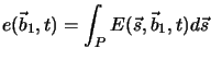
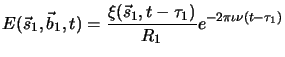
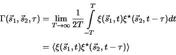
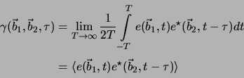
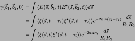
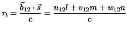
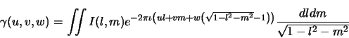
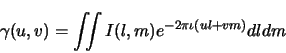
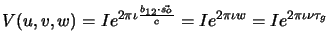
![$\displaystyle V(u,v,w) = I(l,m) \left[ \cos (2 \pi {D \over
\lambda} \sin(\theta(t))) + \iota \sin (2 \pi {D \over \lambda}
\sin(\theta(t))) \right]$](img323.png)
![\includegraphics[]{Ant_Csq.eps}](img357.png)
![$\displaystyle \phi=2\pi{\nu^o_{RF} \over c} \left[\Delta X\cos(\delta)\cos({\it...
...cos(\delta)\sin({\it H}) + \Delta Z\sin(\delta)\right] + 2\pi\tau_{Fix}\nu_{IF}$](img450.png)