In practice, however, the antenna based amplitude
(
![]() ) and phase (
) and phase (![]() ) are potentially time
varying quantities. This could be due to changes in the ionosphere,
temperature variations, ground pick up, antenna blockage, noise pick
up by various electronic components, background temperature, etc.
Treating the quantities under the square root in the above equation as
the antenna dependent amplitude gains, these can be written as complex
gains
) are potentially time
varying quantities. This could be due to changes in the ionosphere,
temperature variations, ground pick up, antenna blockage, noise pick
up by various electronic components, background temperature, etc.
Treating the quantities under the square root in the above equation as
the antenna dependent amplitude gains, these can be written as complex
gains
![]() where
where
![]() . For
an unresolved source at the phase tracking center, variations in this
amplitude will be indistinguishable from a variations in the ratio of
. For
an unresolved source at the phase tracking center, variations in this
amplitude will be indistinguishable from a variations in the ratio of
![]() and
and ![]() .
.
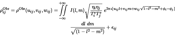
In terms of ![]() s, we can write Equation D.1 as
s, we can write Equation D.1 as
| (15.2) |
 |
(15.3) |
For an unresolved source at the phase tracking center, all terms in
the exponent of
![]() are exactly zero.
are exactly zero.
![]() in this case would be proportional to the flux density of the source.
in this case would be proportional to the flux density of the source.
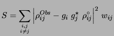
Assuming that the antenna dependent complex gains are independent,
with a gaussian probability density function (this implies that the
real and imaginary parts are independently gaussian random processes),
one can estimate ![]() s by minimizing, with respect to
s by minimizing, with respect to ![]() s, the
function
s, the
function ![]() given by
given by
 |
(15.4) |
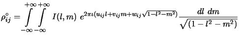
Dividing the above equation by
![]() (the source model,
which is presumed to be known - it is trivially known for an
unresolved source), and writing
(the source model,
which is presumed to be known - it is trivially known for an
unresolved source), and writing
![]() , we get
, we get
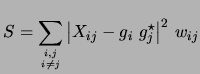
Expanding Equation D.5, we get
![$\displaystyle S=\sum_{{i,j} \atop {i \ne j}}\left[ \left\vert X_{ij}\right\vert...
...X_{ij} - g_i g_j^\star X_{ij}^\star + g_i g_i^\star g_j g_j^\star\right] w_{ij}$](img1140.png) |
(15.6) |
![$\displaystyle {\partial S \over \partial g_i^\star} = \sum_{j \atop {j \ne i}}\left[-g_j X_{ij} w_{ij} +g_i g_j g_j^\star w_{ij}\right] = 0$](img1143.png) |
(15.7) |
This can also be derived by equating the partial derivatives of ![]() with respect to real and imaginary parts of
with respect to real and imaginary parts of ![]() as shown in
Section D.3.
as shown in
Section D.3.
Since the antenna dependent complex gains also appear on the
right-hand side of Equation D.8, it has to be solved
iteratively starting with some initial guess for ![]() s or
initializing them all to 1.
s or
initializing them all to 1.
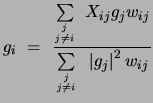
Equation D.8 can be written in the iterative form as:
(the change in ![]() from one iteration to another) where
from one iteration to another) where ![]() is
the tolerance limit.
is
the tolerance limit.
![$\displaystyle g_i^n = g_i^{n-1} + \alpha\left[g_i^{n-1}-{\sum\limits_{j \atop {...
...sum\limits_{j \atop {j \ne i}} \left\vert g_j^{n-1}\right\vert^2 w_{ij}}\right]$](img1145.png)