Algorithm and simulation

In the absence of any polarization leakage, $g_i$s can be estimated by minimizing

$$S = \sum_{{i,j} \atop {i \ne j}}{\left\vert X_{ij}^{{pp}}- {g_i^{\it p}}{g_j^{\it p}}^\star\right\vert}^2 w_{ij}^{{\it p}{\it p}}$$ (10.4)

with respect to $g_i$s, where $w_{ij}^{{\it p}{\it p}}=1/\sigma^2_{ij}$, $\sigma_{ij}$ being the variance on the measurement of $X_{ij}^{{pp}}$.

In Equation 7.2, if ${\rho_{ij,\circ}^{{\it p}{\it p}}}$ accurately represents the source structure, $X_{ij}^{{pp}}$ will have no source structure dependent terms and is purely a product of two antenna dependent complex gains. For a resolved source, ${\rho_{ij,\circ}^{{\it p}{\it p}}}$ can be estimated from the image of the source.

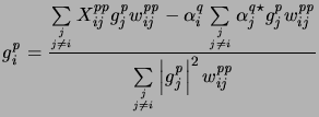
Evaluating $\frac{\partial S}{\partial {g_i^{\it p}}^\star}$ and equating it to zero^10.2(see Appendix D), we get

$${g_i^{\it p}} = {\sum\limits_{j \atop {j \ne i}} X_{ij}^{{pp}}{g_... ... \atop {j \ne i}} \left\vert{g_j^{\it p}}\right\vert^2 w_{ij}^{{\it p}{\it p}}}$$ (10.5)

This can also be derived by equating the partial derivatives of $S$ with respect to real and imaginary parts of ${g_i^{\it p}}^\star$.

Since the antenna dependent complex gains also appear on the right-hand side of Equation 7.5, it has to be solved iteratively starting with some initial guess for $g_j$s or initializing them all to 1. Equation 7.5 can be written in the iterative form as:

$${g_i^{\it p}}^{,n} = {g_i^{\it p}}^{,n-1} + \lambda\left[{g_i^{\i... ...i}} \left\vert{g_j^{\it p}}^{,n-1}\right\vert^2 w_{ij}^{{\it p}{\it p}}}\right]$$ (10.6)

where $n$ is the iteration number and $0 < \lambda < 1$. Convergence would be defined by the constraint $\left\vert S_n-S_{n-1}\right\vert < \beta$ (the change in $S$ from one iteration to another) where, $\beta$ is the tolerance limit and must be related to the average value of $\epsilon_{ij}$. Equation 7.6 forms the central engine for the classical antsol algorithm used for primary calibration of the visibilities and in self-calibration for imaging purposes. This algorithm was suggested by Thompson & D'Addario (1982).

The leaky antsol

In the presence of significant polarization leakage, Equation 7.3 can be used to re-write Equation 7.4 as

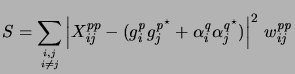$$S = \sum_{{i,j} \atop {i \ne j}} {\left\vert X_{ij}^{{pp}}-( {g^{... ...ha^{\it q}_i \alpha_j^{{\it q}^\star}} ) \right\vert}^2 w_{ij}^{{\it p}{\it p}}$$ (10.7)

In this form, $S$ is an estimator for the true closure noise $\epsilon_{ij}$ rather than the artificially increased closure noise ( ${\alpha_i^{\it q}}{\alpha_j^{\it q}}^\star+\epsilon_{ij}$) due to the presence of polarization leakage.

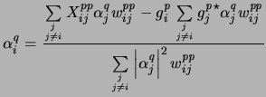
Equating the partial derivatives $\frac{\partial S}{\partial {{g_j^{\it p}}}^\star}$, $\frac{\partial S}{\partial {{\alpha_j^{\it q}}}^\star}$ to zero, we get

$${g_i^{\it p}}= { \sum\limits_{j \atop {j \ne i}}X_{ij}^{{pp}}{g_j... ... \atop {j \ne i}}\left\vert {g_j^{\it p}}\right\vert^2 w_{ij}^{{\it p}{\it p}}}$$ (10.8)

$${\alpha_i^{\it q}}= { \sum\limits_{j \atop {j \ne i}}X_{ij}^{{pp}... ...p {j \ne i}}\left\vert {\alpha_j^{\it q}}\right\vert^2 w_{ij}^{{\it p}{\it p}}}$$ (10.9)

These non-linear equations can also be iteratively solved.

Equation 7.3, which expresses the observed visibilities on a point source unpolarized calibrator in terms of the gains and leakage coefficients of the antennas, would take the same form if written in an arbitrary orthogonal basis. It is clear that the $g$'s and the $\alpha$'s will change when we change the basis, so this means that the equations cannot have a unique solution. This situation is familiar from ordinary self-calibration, when only relative phases of antennas are determinate, with one antenna acting as an arbitrary reference. For observations of unpolarized sources, we can similarly say that any feed can be chosen as a reference polarization, with zero leakage, and other feeds have gains and leakages in the basis defined by this reference. Other conventions may be more convenient, as discussed in Section 7.6 which discusses degeneracy in detail.

Results of the simulations

We simulated visibilities with varying fraction of polarization leakage in the antennas to test the algorithm as follows. The antenna based signal and leakage were constructed as $g_i = R_g$ and $\alpha_i =f\cdot R_\alpha$ where $R_g$ and $R_\alpha$ were drawn from the same gaussian random population. The visibility from two antennas $i$ and $j$ was then constructed as $X_{ij} = g_i g_j^\star + \alpha_i \alpha_j^\star + \epsilon_{ij}$ for $0 \le f < 0.1$. This is equivalent to a visibility of an unpolarized point source of unit strength with a complex antenna based gain $g_i$ and leakage $\alpha_i$ of strength proportional to $f$. Equation 7.6 was then used to compute $g_i$ and residual $\chi ^2$ computed as $\chi^2_\mathrm{a} = \sum_{ij} \left\vert 1-\frac{X_{ij}}{g_i g_j^\star}\right\vert^2$. The computed values of ${g_i^{\it p}}$ were then used to compute improved estimates for ${g_i^{\it p}}$ by simultaneously solving for ${g_i^{\it p}}$ and ${\alpha_i^{\it q}}$ using the iterative forms of Equations 7.8 and 7.9. The derived values of ${g_i^{\it p}}$ and ${\alpha_i^{\it q}}$ matched the true values to within the tolerance limit. A new $\chi ^2$ was computed as $\chi^2_\mathrm{l} = \sum_{ij} \left\vert 1-\frac{X_{ij}}{(g_i g_j^\star + \alpha_i \alpha_j^\star)} \right\vert^2$. The values of $\chi^2_\mathrm{a}$ and $\chi^2_\mathrm{l}$ as a function of $f$ are plotted in Fig. 7.1. The two curves become distinguishable when the leakage is significantly greater than $\epsilon_{ij}$ (for $f$ greater than $\sim1$%). After that, the value of $\chi^2_\mathrm{l}$ is consistently lower than $\chi^2_\mathrm{a}$, where the contribution of antenna based leakage has not been removed. Also notice that $\chi^2_\mathrm{l}$ remains constant while $\chi^2_\mathrm{a}$ quadratically increases as a function of $f$. This is due to the fact that antsol treats the antenna based polarization leakage as closure errors resulting in an increased $\chi ^2$ with increasing fractional leakage.

Figure: Figure showing the results of the simulations. The top curve is the value of $\chi ^2$ using the classical antsol ( $\chi^2_\mathrm{a}$). The bottom curve is the value of $\chi ^2$ using the leaky antsol ( $\chi^2_\mathrm{l}$) as a function of the percentage polarization leakage.