The dominant time-varying direction dependent effect in
interferometric imaging using El-Az mount antennas is due to
the rotation of the projected antenna
Primary Beam (PB) on the sky with time. This
azimuthally-asymmetric PB also varies significantly with
frequency. For wide-band continuum imaging, the rotation of
the PB with time and scaling with frequency together
constitute the dominant time- and frequency-varying
direction dependent (DD) gains. The effects of ignoring
these variable gains leads to errors that are
significantly higher than the thermal noise limit of modern
wide-band radio telescopes (like
the EVLA).
Following are some intial results from that test the WB
A-Projection algorithm to correct for the frequency
dependence of the PB (the related paper is in prepration).
|
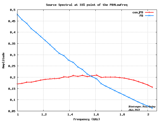
The blue curve shows the
spectrum (covering the frequency range of 1.0 -- 2.0
GHz) of a unit point source located at the ~33% point
of the PB at the reference frequency. The image was
made using the classical imaging algorithm.
|
|

|
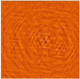
The animations show the simulated PB for the
EVLA at L-Band as a function of frequency (along the
animation axis). The entire animation covers a
frequency range of 1 GHz (Frame 30) to 2 GHz (Frame
1).
|
|
This animation shows the PB-spectra through the 2D
PBs shown in the panels above.
|
Images on this link show the improvements in Stokes-I and -V images after corrections for the PB effects is applied using the A-Projection algorithm.
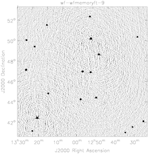
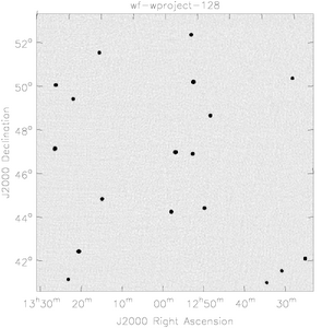
The algorithm to correct for antenna pointing and primary beam effects during imaging was applied to a VLA C-array observation at 1.4GHz (data courtesy Matthews & Uson). The field has two "4C" sources located on either side of the pointing center at roughly the half-power point of the primary beam. Rotation of antenna power pattern on the sky leads to a low level direction dependent error in the Stokes-I image. The Stokes-V power pattern varies much more strongly across the field of view leading to strong direction dependent instrumental Stokes-V error.
The images in the first row below are made using the convectional deconvolution algorithm. Instrumental Stokes-V is clearly visible in the image in the right panel. The peak flux is about 10x higher than the noise limit (~0.1mJy/beam).
The images in the second row were made using the AWProject algorithm. The effects of rotating azimuthally asymmetric primary beams with polarization squint are corrected during image deconvolution. Improvements in imaging performance are clearly visible in both images. There is mild improvement in the Stokes-I image. Improvements in the Stokes-V image are more dramatic. Since we don't expect intrinsic Stokes-V flux for these sources, Stokes-V image should be noise-like. After PB corrections, it is indeed consistent with pure noise.
| Stokes-I image before correction | Stokes-V image before correction |

|

|
| Stokes-I image after correction | Stokes-V image after correction |

|
|
Algorithm to correct for antenna pointing errors and primray beam effects during imaging is reported as EVLA Memo #100 .
Errors in the observed visibilities can be classified as direction dependent and direction independent effects. Since direction dependent effects change arcoss the field of view, they must be corrected during imaging.
Antenna primary beams are usually not azimuthally symmetric due to blockages from feed/feed-legs, etc. As a result, for El-Az mount antennas, sources close to the null and those in the sidelobes experience large gain variations as a function of feed Parallactic angle. As result, these sources are poorly deconvolved and in-beam dynamic range is limited by the PSF sidelobes due to these sources.
Using appropriate Fourier plane filters as part of the forward (data to image) and inverse (image to data) transforms, large scale Primary Beam effects like the VLA polarization squint, antenna pointing errors, etc. can be corrected for a full beam polarimetric imaging experiment. In the example below we used a model for the VLA illumination pattern to construct the Fourier plane filters and correct for the polarization squint, pointing offsets and the effects of rotating primary beam sidelobes for a typical L-band VLA observation.
|
VLA Aperture Illumination pattern @1.4GHz (Courtesy W.Brisken, EVLA Memo #58 ) |
Primary Beam projected on the sky as a function of time |
|
|
Shown below are results from VLA L-band simulations. The first sidelobe was included in the imaging. Stokes-I and -V images are corrected for VLA polarization squint and PB rotation on the sky. The images on left are not corrected for antenna pointing errors.
| Stokes-I before pointing correction | Stokes-I image after pointing correction |
|
|
| Stokes-V before pointing correction | Stokes-V image after pointing correction |
|
|
| Peak residual and RMS for this image is ~50μJy and ~10μJy respectively |
Peak residual and RMS for this image is ~5μJy and ~1μJy respectively |
Algorithm to solve for antenna based pointing errors is reported as EVLA Memo #84 .
-
The imaging dynamic range of an aperture synthesis telescope
for mosaicing and for fields with significant flux throughout
the antenna primary beams can be limited by the knowledge of
the individual primary beams projected on the sky. For high
dynamic range imaging of such fields, one requires an accurate
measurement of the shape of the primary beams and the pointing
offsets as a function of time. The effect of antenna pointing
errors remain separable in the visibility domain. With at
least two, well separated sources along the RA and Dec axis
each to constrain the solutions, it is possible to solve for
these errors in an antenna based fashion in the visibility
domain.
We analyzed the effect of antenna based pointing errors on the imaging dynamic range and fidelity and present an algorithm to solve for these errors using a model for the sky brightness distribution. For a typical L-band eVLA simulation with typical pointing errors for the VLA antennas, the RMS noise can be reduced by a factor of ∼10 using this algorithm. The improvement in the image fidelity is even larger. The formulation given here can be further extended to include other direction dependent effects - specially for application to mosaicing observation. Extension of this work for such, more sophisticated solvers is in progress.
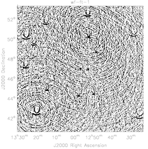
Pointing error solution Residuals: Before correction Residuals: After correction 

Antenna pointing errors as a function of time (continuous lines). Dashed lines show the residual pointing errors after Pointing Selfcal Residual image before pointing correction. The peak and RMS noise in the image is ~250μJy/beam and ~15μJy respectively. Residual image after pointing correction. The peak and RMS noise in the image is ~5μJy/beam and ~1μJy respectively.
Here is the link to our paper on Adaptive Scale Pixel(Asp)-model deconvolution which is an adaptive scale sensitive algorithm. The algorithm is implemented as a Glish client in AIPS++ and is currently been incorporated in the imager tool.
-
Deconvolution of the telescope Point Spread Function (PSF) is necessary for even moderate dynamic range imaging with interferometric telescopes. The process of deconvolution can be treated as a search for a model image such that the residual image is consistent with the noise model. For any search algorithm, a parameterized function representing the model such that it fundamentally separates signal from noise will give optimal results. In general, spatial correlation length (a measure of the scale of emission) is a stronger separator of the signal from the noise, compared to the strength of the signal alone. Consequently scale sensitive deconvolution algorithms result into more noise-like residuals.
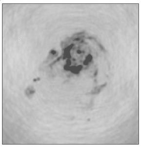
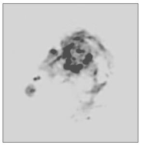
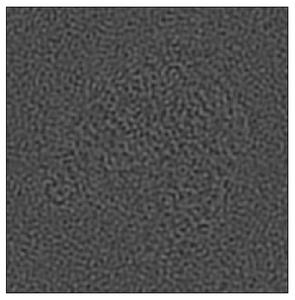
Shown below is an example of the performance of the Adaptive Scale Pixel (Asp) deconvolution algorithm. The first image below is the Dirty Image for a complex source. The image was deconvolved using the Asp-Clean algorithm and the restored image is shown in the second panel below. The residual image, shown in the third panel is consistent with random noise with no correlated features larger than the resolution element.
The Dirty Image The restored image The residual image