2 Examples

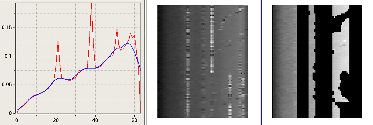
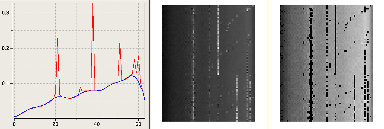
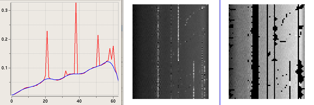
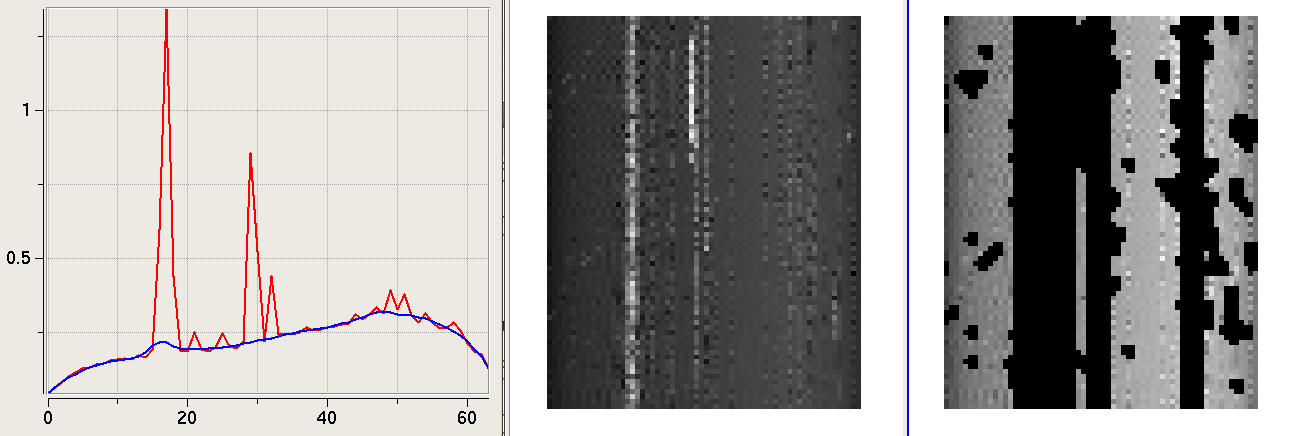
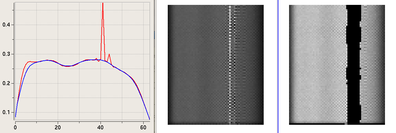
Below are a few examples. The left panels show a plot of the average bandpass per ntime x nchan chunk. The data is shown in red, and the piece-wise polynomial fit is shown in blue. Ideally, the blue line should be a smooth fit across the base of RFI spikes. The middle and right panels show the data ('expr' applied to 'column') as a function of channel number (on the x-axis) and time (on the y-axis). The middle panels show only the data, and the right panels show data with flags (shown in black).

These examples are taken from an L-Band EVLA dataset taken with 1-second integrations and 1-MHz channel resolution.

2.1 Flag Levels 0,1,2 (spw 9 : 1.01 - 1.08 GHz)

These three plots suggest that level 1 is most appropriate for moderate RFI.

FLAG LEVEL 0 : Flagged 8% : tfcrop.flag('Four_ants_3C286.ms',spw='9',baseline='1&2',flaglevel=0,maxnpieces=7,ntime=80)

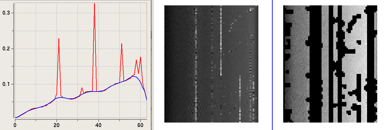
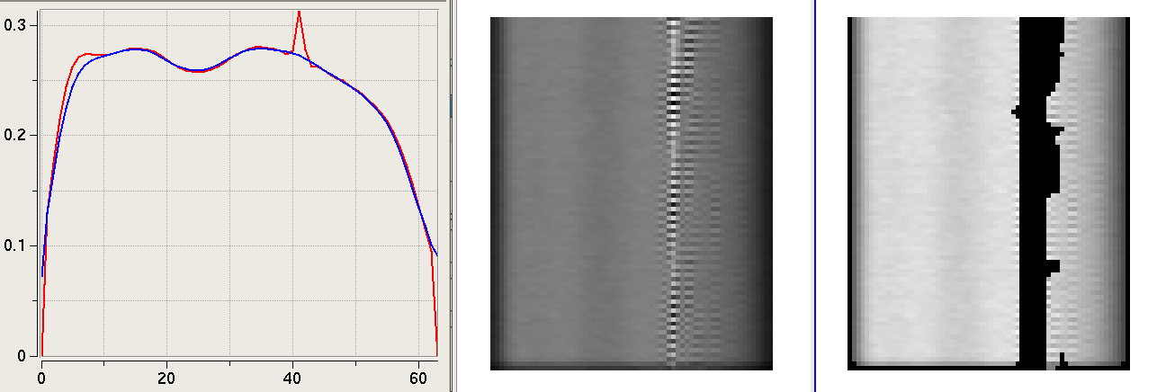
FLAG LEVEL 1 : Flagged 19% : tfcrop.flag('Four_ants_3C286.ms',spw='9',baseline='1&2',flaglevel=1,maxnpieces=7,ntime=80)

FLAG LEVEL 2 : Flagged 44% : tfcrop.flag('Four_ants_3C286.ms',spw='9',baseline='1&2',flaglevel=2,maxnpieces=7,ntime=80)

2.2 Flag Levels 0,1,2 (spw 10 : 1.08 - 1.15 GHz)

When there is a LOT of RFI, flag-level 2 may be most appropriate.

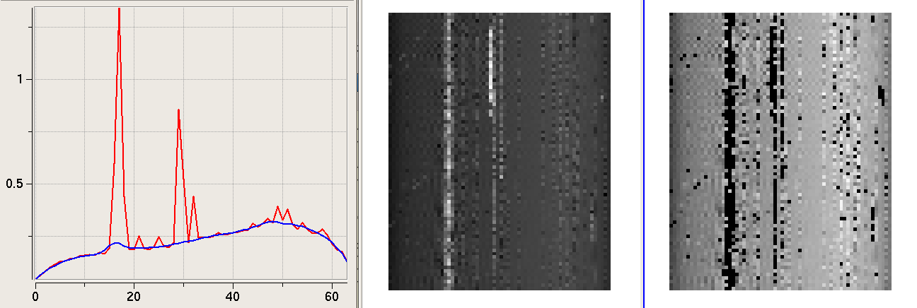
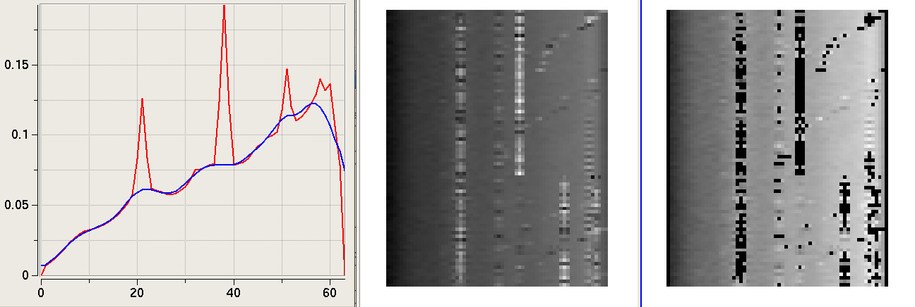
FLAG LEVEL 0 : Flagged 9% : tfcrop.flag('Four_ants_3C286.ms',spw='10',baseline='2&3',flaglevel=0,maxnpieces=7,ntime=80)

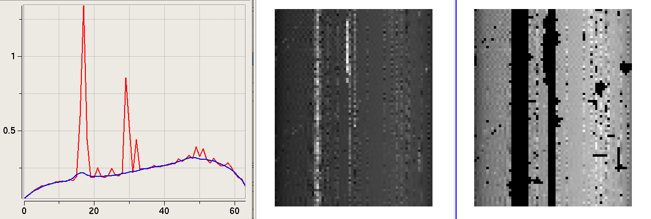
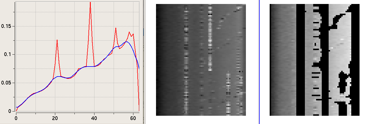
FLAG LEVEL 1 : Flagged 19% : tfcrop.flag('Four_ants_3C286.ms',spw='10',baseline='2&3',flaglevel=1,maxnpieces=7,ntime=80)

FLAG LEVEL 2 : Flagged 47% : tfcrop.flag('Four_ants_3C286.ms',spw='10',baseline='2&3',flaglevel=2,maxnpieces=7,ntime=80)

2.3 Channel selection (spw 6 : 2.02 - 2.08 GHz)

This pair of plots give an example where the piecewise polynomial fit (blue line) may not be accurate, and result in flagging good data. This can be fixed by changing the maximum number of pieces in the polynomial, or be preflagging (or excluding) the end channels.

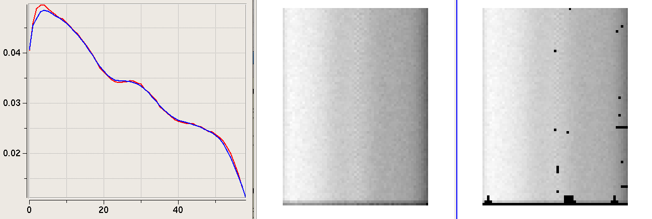
ALL CHANNELS : Flagged 15% : tfcrop.flag('Four_ants_3C286.ms',spw='6',expr='ABS RR',flaglevel=1,maxnpieces=7,ntime=80,baseline='0&2'); This is an example of the polynomial fit failing at the edge of the band, and data being unnecessarily flagged.

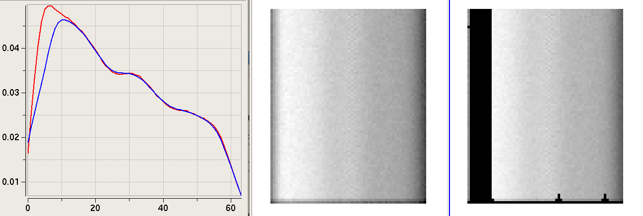
WITHOUT END CHANNELS : Flagged 2% : tfcrop.flag('Four_ants_3C286.ms',spw='6:3 61',expr='ABS RR',flaglevel=1,maxnpieces=7,ntime=80,baseline='0&2'); The polynomial fit is better at the edges.

2.4 Using pre-existing flags (usepreflags=True)

This plot shows an example of flagging on a dataset that already has some flags. Of the gray-scale plots, the left-hand plot contains pre-flags, and the right-hand plot contains all flags (old and new). On the average bandpass plot on the left, the red (data) line has dips (pre-flags) wherever a channel been pre-flagged (for all timesteps in the displayed range). These pre-flagged channels are not included in the bandpass fit (blue).

WITH PRE-EXISTING FLAGS : Old Flags : 12.5% : New Flags : 24.1% : tfcrop.flag('Only_3C286_A.ms',showplots=True,ntime=100,usepreflags=True);

2.5 Effect of Hanning Smoothing - 1 (spw 4, 1.90 - 1.97 GHz)

An example of when Hanning smoothing helps.

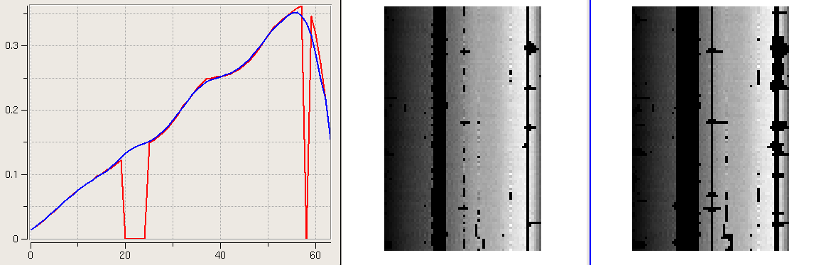
WITHOUT HANNING SMOOTHING : Flagged 15% : tfcrop.flag('Four_ants_3C286.ms',spw='4',baseline='0&1',flaglevel=1,maxnpieces=7,ntime=80); A lot of ringing extending across +/- 10 channels.

WITH HANNING SMOOTHING : Flagged 16% : tfcrop.flag('Hanning_Four_ants_3C286.ms',spw='4',baseline='0&1',flaglevel=1,maxnpieces=7,ntime=80); Less ringing. It has also flagged end-channels, slightly increasing the percentage flagged. Un-selecting end channels can help here.

2.6 Effect of Hanning Smoothing + Flag Levels 0,1,2 (spw 9)

An example of when Hanning smoothing will result in less ringing, but more channels being flagged (compare to the first three plots : spw 9 flaglevels 0,1,2 without Hanning smoothing).

FLAG LEVEL 0 + HANNING : Flagged 12% : tfcrop.flag('Hanning_Four_ants_3C286.ms',spw='9',baseline='1&2',flaglevel=0,maxnpieces=7,ntime=80)

FLAG LEVEL 1 + HANNING : Flagged 35% : tfcrop.flag('Hanning_Four_ants_3C286.ms',spw='9',baseline='1&2',flaglevel=1,maxnpieces=7,ntime=80)

FLAG LEVEL 2 + HANNING : Flagged 54% : tfcrop.flag('Hanning_Four_ants_3C286.ms',spw='9',baseline='1&2',flaglevel=2,maxnpieces=7,ntime=80)

2.7 Example Plots from all SPWs

The first plot shows 15 SPWs in which flagged data (pink) is plotted on top of unflagged data (other colours). The second plot shows only the unflagged data. This is for one baseline and one scan (flaglevel = 1).