2. Currently available Imaging and Deconvolution task-options

This section summarizes a few imaging use-cases, and lists currently supported parameter combinations that control various parts of the image-reconstruction.

Note : This is not a complete list of parameters. Only parameters relevant to choosing imaging and deconvolution are shown. All other parameters apply to whatever combination is set by this listed subset. For example, data selection parameters are independent of those listed below, and parameters such as 'niter','gain','threshold','imsize','cellsize', etc... apply to all the following choices.

2.1 General setup and running

2.1.1 Data and Image Partitioning

mode

'mfs'

Use all channels together

nterms	1	number of terms to use to model the sky frequency dependence
reffreq	' '	reference frequency for the Taylor polynomial

'frequency'

Make a spectral cube (see inline help for subparams)

nchan	-1	nchans in output image
start	0	starting chan/freq
width	' '	bw to average over
interpolation	' '	linear, nearest, cubic
chaniter	True/False	clean each channel to completion separately or not
outframe	'LSRK'	LSRK is the default frame. It can be modfied in the viewer after imaging

Note : channel-averaging using 'width' combined with interpolation='linear','cubic' is currently inconsistent in the code and will be fixed.
Note : chaniter=False uses the first channel's PSF to compute the clean restoring beam, but chaniter=True uses a channel-dependent restoring beam.

'channel'

(almost) same as above

'velocity'

(almost) same as above

'cube'

merges 'channel','frequency','velocity'
Not yet implemented

stokes

'I'

Stokes and correlation options :
I, Q, U, V, IQ, IV, QU, UV, IQU, IUV, IQUV - for Circular and Linear feeds
RR, LL, RRLL - for Circular feeds; XX, YY, XXYY - for Linear feeds

outlierfile

' '

AIPS-style outlier file (a text file with field id, phase-center, and image size for a set of outlier fields)
Multiple fields can also be specified by giving lists for imagename, cell, imsize, phasecenter, mask. This mode has not been tested with all possible combinations of masking and modelimage options.

gridmode

'widefield'

When wprojplanes=1 and facets > 1, a grid of facets is created and deconvolved separately

mask

' '

One or more pixel ranges ( mask=[10,10,20,20] ), region files ( mask=[ 'one.rgn', 'two.rgn'] ), mask-image names ( mask='3c286.mask' ), boxfiles ( mask='boxlist.txt' ) or some combinations of them. If unspecified, it defaults to a full-image of ones.
For multifields, the 'outlierfile' is used to specify masks. When 'imagermode='mosaic', 'minpb' is used to set a primary-beam-based mask irrespective of 'pbcor'=True/False; otherwise, a PB-based mask is made only when 'pbcor'=True.

2.1.2 Controlling number of major/minor cycles

The number of major and minor cycles depend on the choice of total number of iterations (niter), the user supplied stopping threshold (threshold), and the Minor-cycle stopping threshold computed as max(threshold,flux-limit) where flux-limit = current peak residual x PSF sidelobe level. The peak sidelobe level is computed as a fraction of the PSF peak. The additional parameters cyclefactor and cyclespeedup are used to control the number of minor-cycle iterations.

threshold	'0.0mJy'	final stopping threshold
niter	500	maximum number of iterations (across major cycles)
cyclefactor	1.5	flux limit = (peak residual) x (PSF sidelobe level) x cyclefactor A lower cyclefactor will force the minor cycle to clean deeper. If (PSF sidelobe x cyclefactor) > 0.8, fluxlimit = (0.8 x peak residual) to prevent getting a threshold larger than the peak residual
cyclespeedup	-1	If larger than 0, the threshold is increased by pow(2.0, itercount/cyclespeedup). A value larger than zero will cause shallower cleaning than that computed by the flux-limit. Also, for values larger than zero, a higher cyclespeedup causes the minor cycle to clean deeper. [Note: This parameter is currently not treated the same in all algorithms. Its behaviour will either be modified or removed. ]
maxniter	-1	If larger than 0, this is the maximum number of allowed minor-cycle iterations before a major cycle is forced. [Note: Not yet Implemented. Will be added as a clearer alternative to 'cyclespeedup'.]

2.1.3 Imaging and Deconvolution options (summary)

psfmode	'hogbom'	Use the full PSF in minor-cycle updates Accurate but expensive.
	'clark'	Use a radially truncated PSF for minor cycle updates. Approximate but quick for fields of point-sources.
gridmode	' '	Standard Imaging : gridding-convolution function is a prolate spheroidal.
	'widefield'	Wide-field imaging : gridding convolution function is the w-projection kernel.
imagermode	' '	Do only one major cycle, and use 'psfmode' to decide how to use the PSF in the minor cycle iterations
	'csclean'	Do Cotton-Schwab major/minor cycles. Customize with cyclefactor,cyclespeedup. Use psfmode.
	'mosaic'	Mosaic imaging : Pointing offsets are applied via gridding convolution functions. Uses Cotton-Schwab major/minor cycles. Use psfmode.
multiscale	[]	If not empty, use the ms-clean algorithm with the specified list of scale sizes. Ignores 'psfmode'. Will be moved into 'psfmode'. Use the full PSF convolved with multiscale basis functions in minor-cycle updates
pbcor	False	no primary-beam correction
	True	apply image-domain primary-beam correction
Exceptions		psfmode is ignored if gridmode='widefield' or imagermode='mosaic' or multiscale is not []
		The combination of gridmode='widefield' and imagermode='mosaic' is currently not supported
		For nterms>1, imagermode='mosaic' and pbor=True are currently not supported, and psfmode is ignored.

2.2 Specific use-cases

2.2.1 Standard Imaging (narrow-field narrow-band)

Imaging : Standard gridding using a prolate-spheroidal function and natural, uniform or briggs weighting. No direction-dependent corrections.
Deconvolution : Hogbom, Clark, Cotton-Schwab CLEAN Multiscale-CLEAN

mode	'mfs' with nterms=1 (OR) 'channel','frequency','velocity'
gridmode	' ' : use standard gridding
psfmode	'hogbom' : use full PSF (OR) 'clark' : use truncated PSF
imagermode	' ' : one major cycle (OR) 'csclean' : multiple major cycles
multiscale	[] : point-source flux model (OR) [0,6,10] : list of scale sizes in units of pixels If this list is not empty, psfmode is ignored and the ms-clean algorithm uses the full PSF smoothed to the specified scale sizes
pbcor	False : no primary-beam correction

2.2.2 Wide-Field Imaging (direction-dependent corrections)

Imaging : Standard gridding, primary-beam correction (image-domain only), mosaics (with and without pb-correction), w-term correction (faceting or w-projection), all with natural, uniform or briggs weighting.
Deconvolution : Cotton-Schwab CLEAN, multiscale CLEAN.

mode	'mfs' with nterms=1 (OR) 'channel','frequency','velocity'
gridmode	' ' : standard gridding (OR) 'widefield' : faceting or w-projection (wprojplanes>1 and/or facets>1)
psfmode	'hogbom' : use full PSF (OR) 'clark' : use truncated PSF psfmode is ignored if gridmode='widefield' or imagermode='mosaic' or multiscale is not []
imagermode	' ' : one major cycle (OR) 'csclean' : multiple major cycles (OR) 'mosaic' : multiple major cycles, primary-beam correction according to mosaic pointing offsets (psfmode and pbcor are ignored) The combination of gridmode='widefield' and imagermode='mosaic' is currently not supported.
multiscale	[] : point-source flux model (OR) [0,6,10] : list of scale sizes in units of pixels
pbcor	False : no primary-beam correction (OR) True : apply image-domain primary-beam correction If imagermode='mosaic', then irrespective of pbcor, a mask is created using 'pbmin' as a cutoff. It imagermode is not 'mosaic', then a 'pbmin' based mask is created only if 'pbcor=True'.

2.2.3 Wide-Band Imaging (reconstruct sky brightness and spectrum)

Imaging : Standard gridding, w-term correction (w-projection) with natural, uniform or briggs weighting
Deconvolution & MS-MFS (multi-scale multi-frequency synthesis)

mode	'mfs' only, with nterms > 1
gridmode	' ' : standard gridding (OR) 'widefield' : w-projection only (wprojplanes>1 and facets=1)
psfmode	Ignored. multiscale is always used.
imagermode	Ignored. Multiple major cycles are always used. An adaptive flux limit is used per major cycle. Mosaic mode is not yet supported for wideband imaging
multiscale	[] : point-source flux model (OR) [0,6,10] : list of scale sizes in units of pixels
pbcor	False : no primary-beam correction PB correction is not yet supported for wideband imaging

2.3 ARDG work in progress

1. Use A-projection, w-projection and gridded-mosaicing simultaneously.
2. Combine MS-MFS with AW-projection, and gridded-mosaicing (wide-band wide-field imaging)
3. Correction of full-Stokes PB effects (full-Stokes A-projection)
4. MS-MFS for Stokes Q,U,V.

2.4 Imager Class Diagrams - old Imager

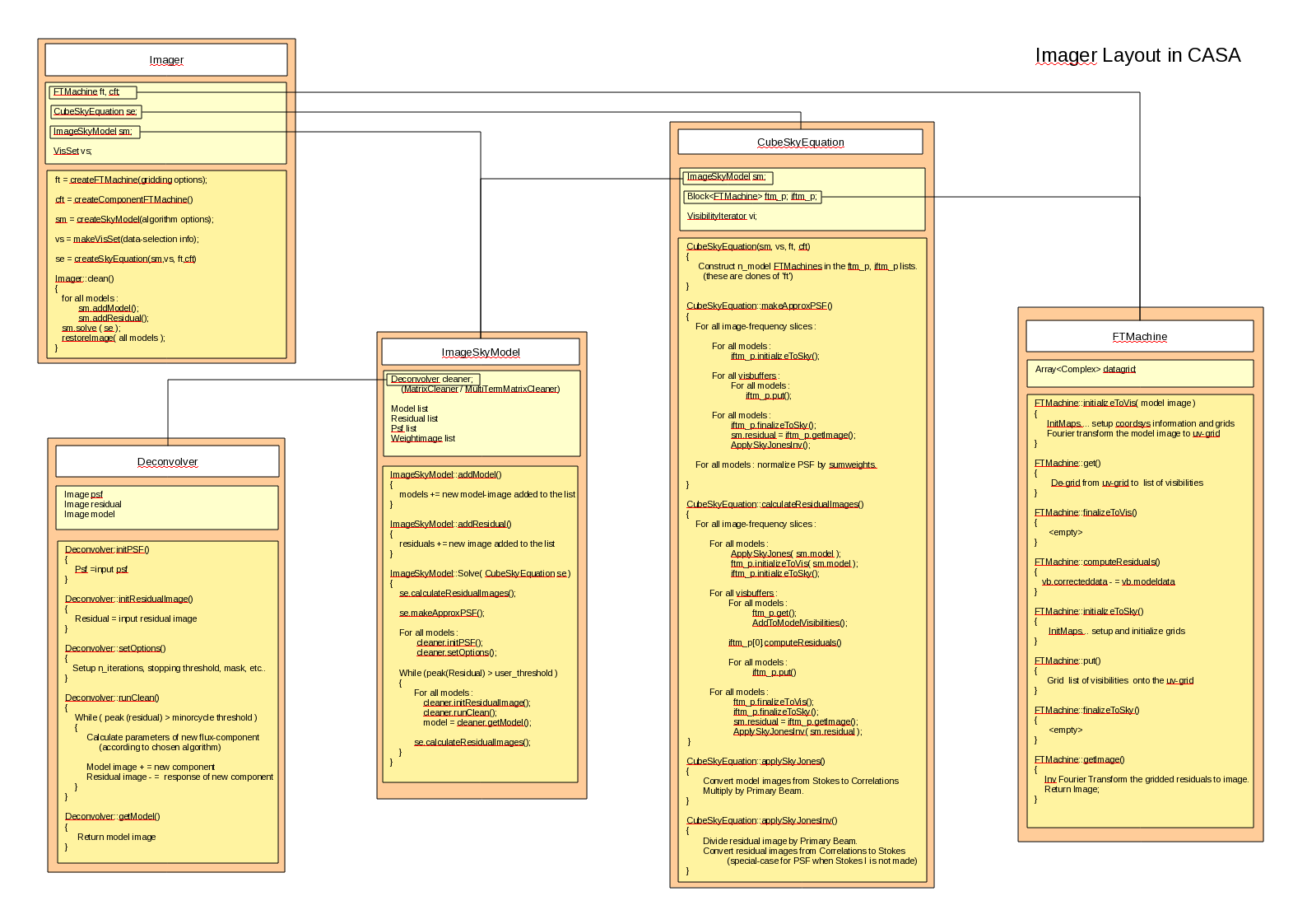
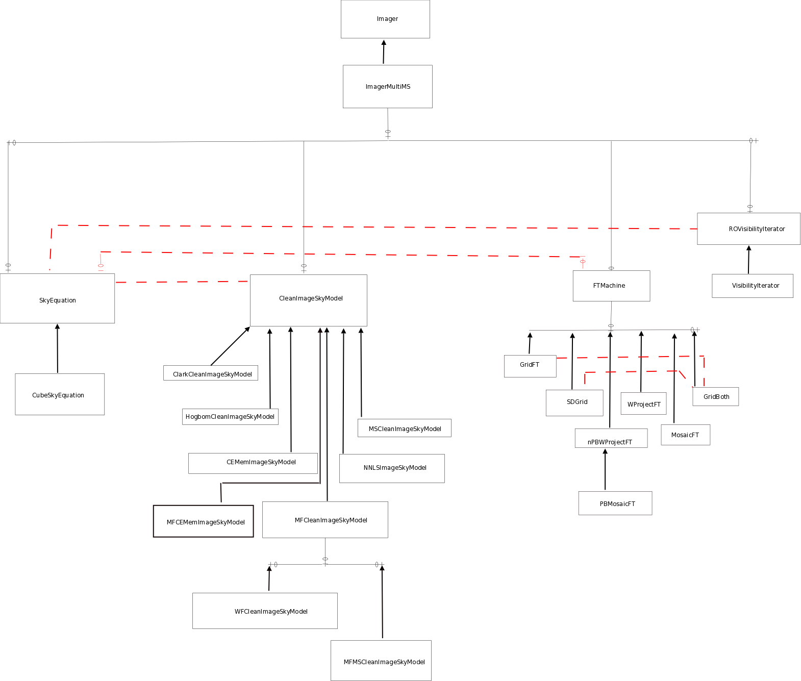
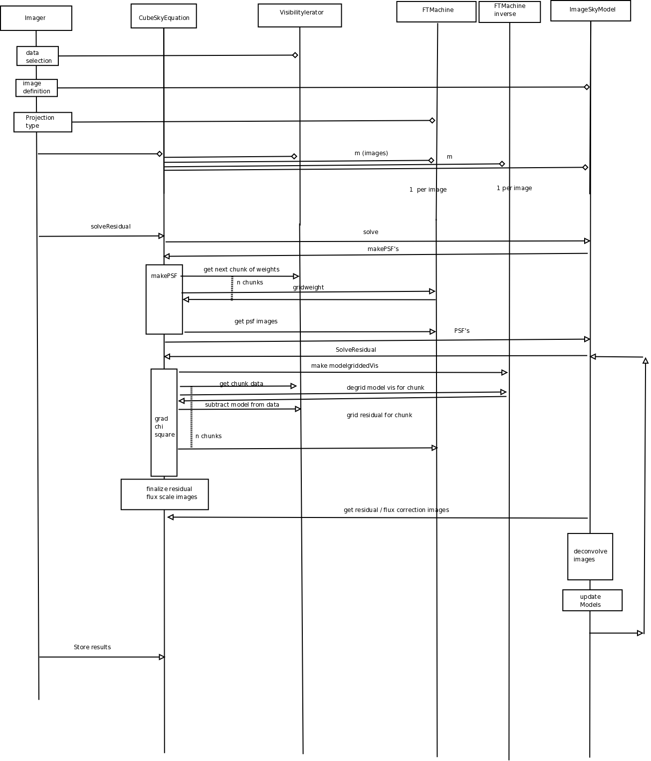
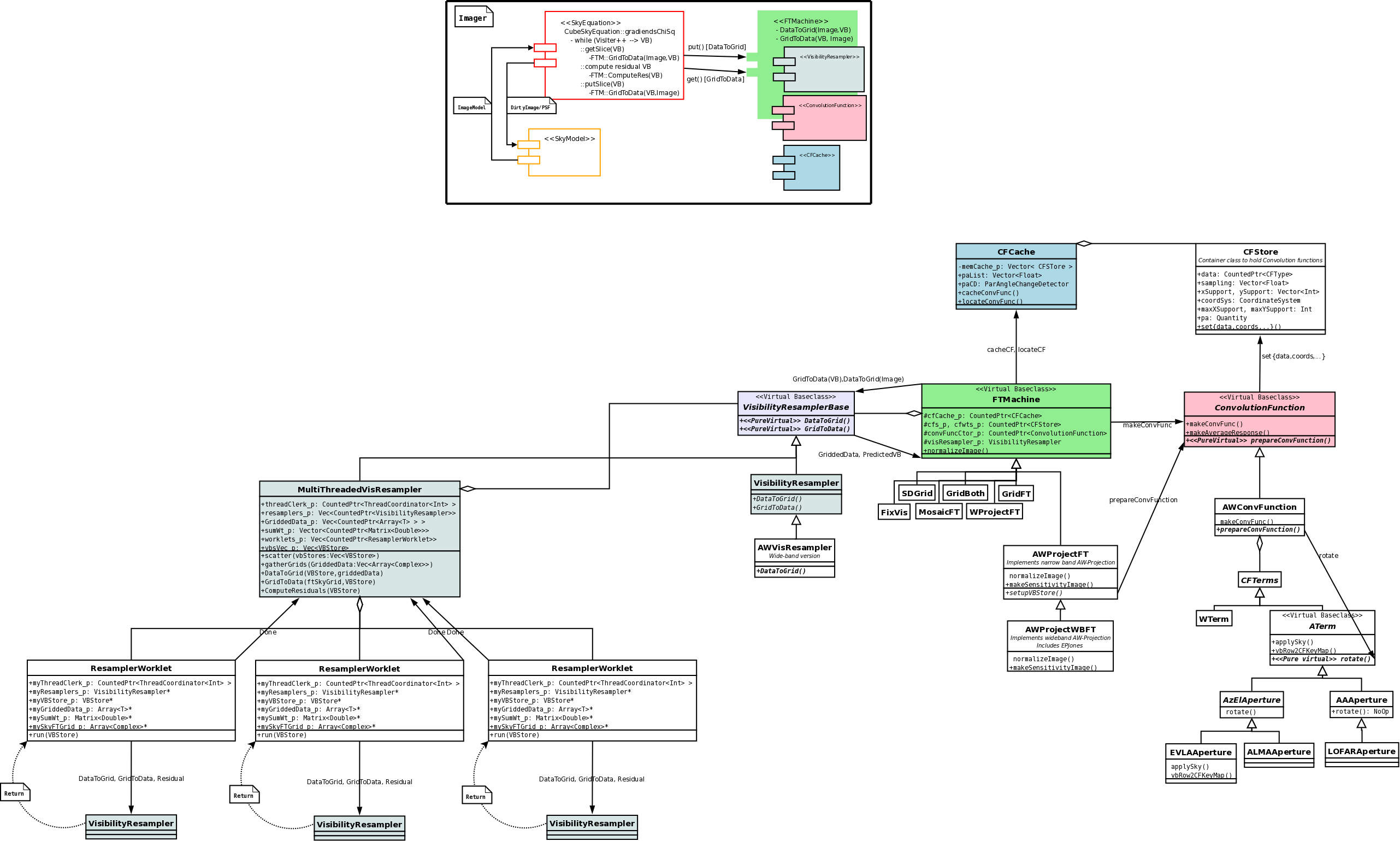
Here are a few diagrams to convey the layout and flow-of-control within the Imager-module classes.

1. Imager Layout and Control-Flow : A (May 2011) summary of the basic flow of control within the Imager classes for major/minor cycles and gridding/degridding (written as pseudo-code).

   Note : This diagram shows the main calls that are common to all derivatives of ImageSkyModels and FTMachines. The actual code tree has much more code for many special-cases controlled by various state variables. Various set-up functions are not listed. There are also some naming differences between the diagram and code : The function CubeSkyEquation::calculateResidualImages() is actually CubeSkyEquation::gradientsChiSquared() in the code. Also, ImageSkyModel::solve() is in some cases, ImageSkyModel::solveResiduals(). The Deconvolver interface is not consistent across all minor-cycle algorithms.

2. Imager Hierarchy and Imager Control Flow (from K.Golap) : A (May 2010) summary of the Imager/ImageSkyModel/FTMachine class hierarchy and function-call sequence.

3. FTMachine Hierarchy (from S.Bhatnagar) : A (May 2011) class diagram of the FTMachine, ConvolutionFunction, and Resampler classes.

2.5 Spectral Reference Frames in the current/old Imager/Clean

CASA images contain an intrinsic spectral reference frame, plus an optional conversion layer that relabels the frequency coordinates in other frames. Tools like the Viewer can also apply on-the-fly conversions to relabel frequencies in frames other than what the image contains.

Internal to Imager, the gridding process operates entirely in the LSRK frame. Data channel frequencies are converted to LSRK via vb.lsrfrequency() and compared with image channel frequencies also in LSRK, to determine the mapping between data channels and image channels. For the data, this is a time-dependent relabelling of the frequencies ( if the data are not already in LSRK/REST ).

1. When used from the tool level, the images are always created in the LSRK frame. The freqstart, freqstep, freqframe parameters in im.defineimage() define the parameters of the spectral coordinate system in the units the user wishes to express them. These values are internally converted to LSRK frequencies, before creating the images. Output images are in LSRK frequencies with no extra conversion layer. The Viewer, by default, will show images in LSRK, and the user must apply an on-the-fly conversion via the Viewer adjust panel, to see it in any other frequency frame, or in velocities.

2. When used from the clean task, the images are created in the user-specified output frame, in the python code. If unspecified, it picks the frame from the MS. Internally in Imager2.cc, a conversion layer to LSRK is set, to allow the gridding to work correctly in LSRK. In python again, at the end of the clean task, this conversion layer is deleted, resulting in an image in the user-requested output frame with no extra conversion layer. The Viewer, by default, will show images in the user-chosen output frame.

This difference in behaviour has caused some confusion, and we plan to synchronize things. To the end user, however, both these options give the same results when Viewed with the appropriate output frame in the Viewer.

Note that Conversions to TOPO or GEO represent a single time within the observation ( our convention is the start time of the dataset ). If the dataset is also TOPO or GEO, this will not be a one-to-one mapping between data channels and image channels ( a common source of user confusion ). A true one-to-one mapping is possible only if the MS frame is redefined as 'REST' so that no time-dependent LSRK conversion is done internally.