


Next: 2. Currently available Imaging
Up: Imaging Algorithms in CASA
Previous: Contents
Contents
Subsections
1.1 Imaging
Imaging is the process of converting a list of calibrated visiblities into a raw or 'dirty' image.
There are three stages to inteferometric image-formation : weighting, convolutional resampling, and a Fourier transform.
During imaging, the visibilities can be weighted in different ways, to alter the instrument's natural response function in ways that make the image-reconstruction tractable.
- Natural :
The natural weighting scheme gives equal weight to all samples. Usually, lower spatial frequencies are sampled more often than the higher ones, producing an uneven signal-to-noise ratio across the spatial-frequency plane. This can sometimes result in undesirable structure in the PSF which reduces the accuracy of the minor cycle. However, at the location of a source, this method preserves the natural peak sensitivity of the instrument.
- Uniform :
Uniform weighting gives equal weight to each measured spatial frequency irrespective oaf sample density.
The resulting PSF has a narrow main
lobe and suppressed sidelobes across the entire image and is best suited for sources with
high signal-to-noise ratios to minimize sidelobe contamination between sources. However,
the peak sensitivity is much less than optimal, since data points in densely sampled regions
have been weighted down to make the weights uniform. Also, isolated measurements can
get artifically high relative weights and this may introduce further artifacts into the PSF.
- Briggs :
Briggs or Robust weighting ([Briggs 1995]) creates a PSF that smoothly
varies between natural and uniform weighting based on the signal-to-noise ratio of the
measurements and a tunable parameter that defines a noise threshold. High signal-to-noise
samples are weighted by sample density to optimize for PSF shape, and low signal-tonoise
data are naturally weighted to optimize for sensitivity.
- uv-Taper :
uv-tapering applies a multiplicative Gaussian taper to the spatial frequency
grid, to weight down high spatial-frequency measurements relative to the rest. This suppresses
artifacts arising from poorely sampled regions near and beyond the maximum spatial
frequency. This is important for deconvolution because visibilities estimated for these
regions would have poor or no constraints from the data. Also, the natural PSF is smoothed
out and this tunes the sensitivity of the instrument to scale sizes larger than the
angular-resolution of the instrument by increasing the width of the main lobe. uv-tapering
is usually applied in combination with one of the above weighting methods.
Imaging weights and weighted visibilities are first resampled onto a regular uv-grid (convolutional resampling) using a prolate-spheroidal function as the gridding convolution function (GCF). The result is then Fourier-inverted and grid-corrected to remove the image-domain effect of the GCF. The PSF and residual image are then normalized by the sum-of-weights.
Older methods use standard imaging along with image-domain operations to correct for direction-dependent effects. Newer methods apply direction-dependent,time-variable and baseline-dependent corrections during gridding in the visibility-domain, by choosing/computing the appropriate GCF to use along with the imaging-weights.
For wide-field imaging, sky curvature and non-coplanar baselines result in a non-zero w-term. Standard 2D imaging applied to such data will produce artifacts around sources away from the phase center. There are three methods to correct the w-term effect.
- Image-plane faceting : Multiple image-domain facets are created by gridding the visibilities multiple times for different phase-reference centers. These facets are deconvolved separately using their own PSFs. Model images from all facets are used to predict a single set of model visibilities, from which a new set of residual-image facets are computed. One disadvantage of this method is that emission that crosses facet boundaries will not be deconvolved accurately. (Ref : Cornwell & Perley 1992, 1999).
- UV-domain faceting : Visibilities are gridded multiple times onto the same uv-grid, each time with a different phase-reference center. One single dirty/residual image is constructed from the resulting grid and deconvolved using a single PSF. Unlike in image-domain faceting, this deconvolution is not affected by emission that crosses facet boundaries. (Ref : Sault et al, 1999)
- W-projection : Visibilities with non-zero w-values are gridded using using a GCF given by the Fourier transform of the Fresnel EM-wave propagator across a distance of w wavelengths. In practice, GCFs are computed for a finite set of w-values (wprojplanes) and applied during gridding. W-projection is roughly an order of magnitude faster than faceted imaging because it grids each visibility only once. (Ref: Cornwell et al, 2008)
The aperture-illumination-function (AIF) of each antenna results in a direction-dependent complex gain that can vary with time and is usually different for each antenna. The resulting antenna power pattern is called the primary beam. There are two methods to correct for the effect of the primary beam.
- Image-domain PB-correction : A simple method of correcting the effect of the primary beam is a post-deconvolution image-domain division of the model image by an estimate of the average primary beam. This method ignores primary-beam variations across baselines and time, and is therefore approximate, limiting the imaging dynamic-range within the main lobe of the beam to about
 .
.
- A-projection : Time and baseline-dependent corrections are applied during gridding, by computing GCFs for each baseline as the convolution of the complex conjugates of two antenna aperture illumination functions. An additional image-domain normalization step is required, and can result in either a flat-sky or flat-noise image. The advantage of this method is that known time and baseline variability can be accounted for, both during gridding as well as de-gridding. (Ref: Bhatnagar et al, 2008).
Flat Sky vs Flat Noise :
There are two ways of normalizing the residual image before beginning minor cycle iterations. One is to divide out the primary beam before deconvolution and the other is to divide out the primary beam from the deconvolved image. Both approaches are valid, so it is important to
clarify the difference between the two.
- Flat-noise : Primary-beam correction is not done before the minor cycle deconvolution.
The dirty image is the instrument's response to the product of the sky and the primary beam, and therefore the
model image will represent the product of the sky brightness and the average primary beam. The noise in the image is related directly to the
measurement noise due to the interferometer, and is the same all across the image.
The minor cycle can give equal weight to all flux components that it finds.
At the end of deconvolution, the primary beam must be divided out of the model image.
This form of normalization is useful
when the primary beam is the dominant direction-dependent effect because
the images going into the minor cycle satisfy a convolution equation. It is also
more appropriate for single-pointing fields-of-view.
- Flat-sky : Approximate Primary-beam correction is done on the dirty image, before the minor cycle iterations.
The amplitude of the flux components found during deconvolution will be free of the primary beam, and will represent the true sky.
However, the image going into the
minor cycle will not satisfy a convolution equation and the noise in the dirty
image will be higher in regions where the primary-beam gain is low. Therefore, the minor cycle needs to
account for this while searching for flux components (a signal-to-noise dependent
CLEAN). This form of normalization is useful for mosaic imaging where
the sky brightness can extend across many pointings.
This is because mosaic observations are done for sources with spatial
scales larger than the field-of-view of each antenna, and therefore not present
in the data. Allowing the minor cycle to use flux components that span across
beams of adjacent pointings is likely to provide a better constraint on the reconstruction
of these unmeasured spatial frequencies, and produce smoother large-scale emission.
An antenna pointing offset results in a phase-gradient across the aperture illumination function. Ignoring pointing errors of the order of 20 arcsec can limit the imaging dynamic range to
. A known pointing-offset can be corrected during gridding by augmenting the A-projection GCF with a phase-gradient calculated to cancel that due to the pointing offset. Note that the EVLA beam-squint is a polarization-dependent pointing offset, and can also be corrected in this way.
Data from multiple pointings can be combined during gridding to form one single large image.Three methods are currently implemented.
- Linear Deconvolution : Each pointing is deconvolved and the final deconvolved images are stitched together. Heuristics and weights are used to improve the accuracy of deconvolution of emission present in multiple (overlapping) pointings.
- Joint Deconvolution : Dirty/residual images are constructed separately for each pointing, and then weighted and stitched together before deconvolution. The advantage of this method is that deconvolution proceeds on one single image, eliminating the problem of deconvolving emission present in multiple pointings. However, the PSF used during deconvolution will be approximate.
- Mosaic Imaging : Data from each pointing is gridded using a GCF augmented with a phase-gradient (across the spatial-frequency plane) corresponding to the difference between the phase-reference center of the pointing and of the final image. This can be thought of as an intentional pointing-offset. Since this method uses all the visibilities at once and produces one dirty image and one PSF, it has better imaging fidelity (and performance) than linear or joint deconvolution.
1.2 Deconvolution
Deconvolution refers to the process of reconstructing a model of the sky brightness distribution, given a dirty/residual image and the point-spread-function of the instrument. This process is called a deconvolution because under certain conditions, the dirty/residual image can be written as the result of a convolution of the true sky brightness and the PSF of the instrument. Deconvolution forms the minor cycle of iterative image reconstruction in CASA.
The CLEAN algorithm forms the basis for most deconvolution algorithms used in radio interferometry.
The peak of the residual image gives the location and strength of a potential point source.
The effect of the PSF is removed by subtracting a scaled PSF from the residual image at the location of each point source,
and updating the model. Many such iterations of finding peaks and subtracting PSFs form the minor Cycle.
There are several variants of the CLEAN algorithm
In Hogbom CLEAN [Hogbom 1974], the minor cycle subtracts a scaled and
shifted version of the full PSF to update the residual image for each point source. After the
initial dirty image is computed, only minor Cycle iterations are done, making this a purely
image-domain algorithm.
It is computationally efficient but susceptible to errors due to
inappropriate choices of imaging weights, especially if the PSF has high sidelobes.
Clark CLEAN [Clark 1980] also operates only in the image-domaon.
It does a set of Hogbom minor cycle iterations using
a small patch of the PSF. This is an approximation that will result in a speed-up in the minor cycle, but
could introduce errors in the image model if there are bright sources spread over a wide field-of-view where
the flux estimate at a given location is affected by sidelobes from far-out sources.
To minimize this error, the iterations are stopped when the brightest peak in the residual
image is below the first sidelobe level of the brightest source in the initial residual image.
The residual image is then re-computed by subtracting the sources and their responses in the gridded
Fourier domain (to eliminate aliasing errors).
Cotton-Schwab CLEAN [Schwab and Cotton 1983] is similar to the
Clark algorithm, but computes the residual via a full major cycle (use the current image model to predict a list of model visibilities, compute residual visibilities, and grid them to form a new residual image to pass to another set of minor cycles).
It is time consuming but relatively unaffected by preconditioning and gridding
errors because it computes chi-square directly in the measurement domain. It also allows highly
accurate prediction of visibilities without pixelation errors.
Cornwell-Holdaway Multi-Scale CLEAN (CH-MSCLEAN) [Cornwell 2008] is a scale-sensitive deconvolution algorithm designed for images with complicated
spatial structure. It parameterizes the image into a collection of inverted tapered paraboloids.
The minor cycle iterations use a matched-filtering technique to measure the location, amplitude
and scale of the dominant flux component in each iteration, and take into account
the non-orthogonality of the scale basis functions while performing updates.
Multi-Scale Multi-Frequency synthesis (MSMFS) [RaoVenkata 2010] is a wide-band imaging algoorithm that models the wide-band sky brightness distribution as a collection of inverted,tapered paraboloids of different scale sizes, whose amplitudes follow a polynomial in frequency. A linear-least squares approach is used along with standard clean-type iterations to solve for best-fit spectral and spatial parameters.
A point-source version of this algorithm can be run by specifying only one scale size corresponding to a delta-function.
Model the sky brightness distribution as a collection of point-sources. Use a prior image along with an entropy-based penalty function to bias the solution of pixel amplitudes.
The Maximum Entropy method (MEM) [Cornwell and Evans 1985], [Narayan and Nityananda 1986] is a pixel-based deconvolution algorithms that perform
a rigorous constrained optimization in a basis of pixel amplitudes. MEM uses the
Bayesian formulation of chi-square minimization, and applies a penalty function based on relative
image entropy. This choice of penalty function biases the estimate of the
true sky brightness towards a known prior image. If a flat image is chosen as the prior,
the solution is biased towards being smooth, and produces a more realistic reconstruction
of extended emission. Positivity and emptiness constraints can be applied on the image pixels via a
penalty function.
The Adaptive Scale Pixel (ASP) [Bhatnagar and Cornwell 2004]
deconvolution algorithm parameterizes the sky brightness distribution into a collection of
Gaussians and does a formal constrained optimization on their parameters. In the major
cycle, visibilities are predicted analytically with high accuracy. In the minor cycle, the
location of a flux component is chosen from the peak residual, and the parameters of the
largest Gaussian that fits the image at that location are found. The total number of flux-components
is also updated as the iterations proceed.
1.3 Combining imaging, deconvolution and partitioning
The goal of the current algorithm-development effort in CASA is to provide the ability to
match any or all imaging modes (Major cycles with direction-dependent corrections) with any
Minor-cycle deconvolution algorithm.
The end-goal is to enable "Wide-Field Wide-Band Full-Stokes Imaging of emission at multiple spatial scales".
The following is a list of all currently available combinations of imaging and
deconvolution algorithms in CASA, and the resulting functionality.
The visibility data can be partitioned in many ways, with the above algorithms operating independently
on each piece (e.g. one channel at a time, or chunks of channels).
Partitioning can also be done in the image-domain where the same data is used to create
multiple types of images (e.g. Stokes I,Q,U,V, or Taylor-polynomial coefficients or multiple-facets/phase-centers).
- Frequency :
Images can be made for each frequency channel, for groups of frequency channels, or by combining all channels together.
- 'mfs' : Images made by combining data from multiple channels use multi-frequency-synthesis to grid visibilities according to their respective observing frequencies. The frequency at which the output image is created is the middle of the sampled frequency range.
- 'spectral cubes' : For spectral cube options, the desired grid of image frequencies may be set slightly different from the frequencies at which the data were observed. This is to allow output spectral cubes that can remain consistent across observations that may have varying frequency settings. Visibilities used for imaging each output target channel are computed by interpolating between measurements made at nearby frequencies. Options for interpolation include 'nearest' (pick the value at the nearest measured frequency and assume that it is the same as the target frequency), 'linear' (interpolate between measurements on either side; this can be ambiguous when only one adjacent channel has valid data in it), and 'cubic' (cubic interpolation between the three nearest frequencies). When channel averaging is combined with interpolation, visibilties from the specified number of data channels (width) are first interpolated to lie on a frequency-grid centered on the output channel frequency, and then 'mfs' is performed for all channels being combined by 'width'.
Note : The default (and recommended) output frequency reference-frame for spectral-cubes is 'LSRK'.
More information about Spectral Reference Frames
in a knowledgebase article.
- Stokes Options :
Images can be made for all Stokes parameters and correlation pairs (or all combinations possible with the selected data). This is an image-partitioning, where the same data is used to construct the different imaging products.
The currently allowed options are [I, Q, U, V, IQ, IV, QU, UV, IQU, IUV, IQUV] for Circular and Linear feeds, [RR, LL, RRLL] for Circular feeds, and [XX, YY, XXYY] - for Linear feeds. Currently, if any correlation is flagged, all correlations for that datum are considered as flagged.
Note : Stokes imaging behaviour with partially flagged data, mask-extensions, and different minor-cycle options are work in progress :
CAS-2587
- Multi-Field/Facet Options :
Two types of image-domain partitioning are possible.
- One image from multiple field-ids : Data taken with multiple phase-reference centres can be combined during imaging by selecting data from all fields together (multiple field-ids), and specifying only one output image name and one phase-reference center. If mosaic mode is enabled, attention is paid to the pointing centers of each data-fieldid during gridding. and a primary-beam correction is also done.
- Multiple image-fields from the same set of data (facets and outlier fields) : Irrespective of the phase-reference centers of the selected data, it is possible to specify the phase-reference centers of more than one output image.
-- Faceted imaging is one way of handling the w-term effect. A grid of facet-centers is used to create separate dirty images which can then be deconvolved together, or separately, in the minor cycle, but treated together within the major cycle.
-- Outlier fields can also be specified to make separate images for a few far-out sources. Currently this is triggered either by specifying a list of image parameters (name, phase-center, size, pixel resolution, etc), or by supplying an AIPS-style text file.
- Masks :
Masks are images of zeros and ones that decide regions of the image that the minor-cycle is to operate on (wherever there are ones).
- Specifying masks : Masks can be specified via pixel ranges, region files, mask-image names, boxfiles or some combinations of them. Masks for multi-field imaging (facets and outlier fields) are specified via an outlierfile. Masks can be drawn at run-time (interactively).
- Different minor-cycle behaviour : There are some differences in how masks are interpreted in different algorithms. For example, multi-scale clean smooths the mask by each specified scale-function in order to allow corrections when low-level extended emission spills out of a tight user-set box; Clark-clean applies the Stokes-I mask to all stokes planes because it performs a joint search for emission peaks; the mosaic mode uses a default primary-beam based mask (Note : this is valid only for narrow-band mosaic imaging).
Note : Mask-behaviour cleanup is work in progress : CAS-2737
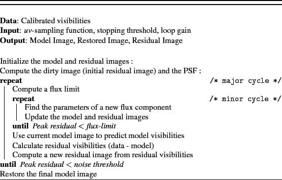
This section describes how Imaging and Deconvolution algorithms are used together.
All iterative image-reconstruction algorithms in CASA use Cotton-Schwab major and minor cycles.
The major cycle computes model and residual visibilities, grids them
via convolutional resampling, and Fourier transforms the result to
form a residual (or dirty) image. This image is interpreted as the
convolution of the sky brightness distribution with the PSF of the
instrument, and the minor cycle deconvolves the PSF from the current
residual image to create a model image.
The Cotton-Schwab cycles proceed as follows:
Single-dish images are constructed using a user-specified convolution function to grid the data onto the image raster. The result is a convolution of the sky by this 'beam'.
Single-dish images can be combined with interferometric images in three ways
- Feathering : Images made separately from single-dish and interferometry data can be combined in a final step. The lower-resolution single-dish image is first re-gridded onto a high-resolution grid corresponding to that of the interferometer image. Both images are Fourier transformed, weighted by taper functions, and added. The result is inverse Fourier-transformed. The taper function used for the single-dish image is FT of the stored primary beam; it is applied only if the image is in units of Jy/pixel. The taper used for the interferometer image is (1 - singledishtaper), so as to retain constant total weight at all uv grid cells.
- Starting model for CLEAN : If there is some overlap in uv-range between the single-dish and interferometric measurements, short-spacing solutions for the interferometric image reconstruction can be constrained by using a single-dish image as a starting model for iterative deconvolution (in units of Jy/pixel and re-gridded to match the resolution of the interferometric image). The single-dish image should be the result of a Wiener deconvolution of the single-dish image by the single-dish primary beam. Approximations to this deconvolution may also suffice if there is sufficient overlap with the interferometer short-baseline measurements.
- Joint deconvolution : To be updated.
Next: 2. Currently available Imaging
Up: Imaging Algorithms in CASA
Previous: Contents
Contents
R. V. Urvashi
2013-10-22