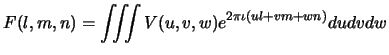
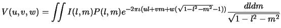
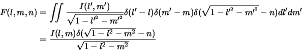
The visibility measured by a properly calibrated interferometer is given by
For a small field of view (
![]() ), the above equation can be
approximated well by a 2D Fourier transform relation. The other case
in which this is an exact 2D relation is when the antennas are perfect
aligned along the East-West direction. Here, we discuss the problem
of mapping with non-East-West arrays. The derivation presented here
of results for devising algorithms used for imaging large fields of
view presented here follow the treatment of
Cornwell & Perley (1992) and Cornwell & Perley (1999).
), the above equation can be
approximated well by a 2D Fourier transform relation. The other case
in which this is an exact 2D relation is when the antennas are perfect
aligned along the East-West direction. Here, we discuss the problem
of mapping with non-East-West arrays. The derivation presented here
of results for devising algorithms used for imaging large fields of
view presented here follow the treatment of
Cornwell & Perley (1992) and Cornwell & Perley (1999).
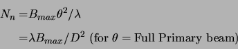
Equation 4.1 also reduces to a 2D relation for a non-East-West array, if the integration time is sufficiently small (snapshot observations). However modern arrays are designed to maximize the uv-coverage with the antennas arranged in a 'Y' shaped configuration (non East-West arrays) (Mathur1969). Fields, such as the ones observed for this dissertation, with emission at all angular scales, require maximal uv-coverage. Telescopes such as the GMRT use the rotation of earth to improve the uv-coverage and observations of complex fields typically last for several hours. Hence, Equation 4.1 needs to be used to map the full primary beam of the antennas, particularly at low frequencies.
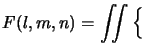
Let
![]() be treated as an independent variable. A 3D
Fourier transform of
be treated as an independent variable. A 3D
Fourier transform of ![]() can be written using (
can be written using (![]() ) and
(
) and
(![]() ) as a set of conjugate variables as
) as a set of conjugate variables as
 |
(7.2) |
 |
 |
||
 |
|||
| (7.3) |
 |
(7.4) |
The effect of including the fringe rotation term (![]() ) would be
a shift of the Image volume by one unit in the conjugate axis
(
) would be
a shift of the Image volume by one unit in the conjugate axis
(![]() axis) (shift theorem of Fourier transforms; Bracewell1986and later eds).
Hence, the effect of fringe stopping is to make the
axis) (shift theorem of Fourier transforms; Bracewell1986and later eds).
Hence, the effect of fringe stopping is to make the ![]() plane coincide
with the tangent plane at the phase center on the Celestial sphere
(the point where the tangent plane touches the Celestial sphere) with
the rest of the sphere completely contained inside the Image
volume (Fig. 4.1).
plane coincide
with the tangent plane at the phase center on the Celestial sphere
(the point where the tangent plane touches the Celestial sphere) with
the rest of the sphere completely contained inside the Image
volume (Fig. 4.1).
![\includegraphics[scale=0.85]{Images/ImgVol.eps}](img576.png)
|
![\includegraphics[]{Images/CelestialProj.eps}](img577.png)
|
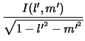
Noting that the third variable ![]() of the Image volume is not an
independent variable and is constrained to be
of the Image volume is not an
independent variable and is constrained to be
![]() ,
Equation 4.5 gives the physical interpretation of
,
Equation 4.5 gives the physical interpretation of ![]() .
Imagine the Celestial sphere defined by
.
Imagine the Celestial sphere defined by
![]() enclosed by
the Image volume
enclosed by
the Image volume ![]() , with the top most plane being
tangent to the Celestial sphere as shown in Fig. 4.1.
Equation 4.5 then tells that only those parts of the Image
volume correspond to the physical emission which lie on the surface
of the Celestial sphere. However, the Image volume will be
convolved by the telescope transfer function. The telescope transfer
function is the Fourier transform of the sampling function
, with the top most plane being
tangent to the Celestial sphere as shown in Fig. 4.1.
Equation 4.5 then tells that only those parts of the Image
volume correspond to the physical emission which lie on the surface
of the Celestial sphere. However, the Image volume will be
convolved by the telescope transfer function. The telescope transfer
function is the Fourier transform of the sampling function ![]() in the
in the
![]() frame (see Chapter 2,
page
frame (see Chapter 2,
page ![]() ). The telescope transfer function,
referred to as the dirty beam and defined as
). The telescope transfer function,
referred to as the dirty beam and defined as
![]() , also defines a volume in the image domain. The dirty image volume defined by the relation
, also defines a volume in the image domain. The dirty image volume defined by the relation
![]() is a convolution of
is a convolution of ![]() with
with ![]() . Since
the dirty beam is not constrained to be finite only on the
Celestial sphere,
. Since
the dirty beam is not constrained to be finite only on the
Celestial sphere, ![]() will be finite away from the surface of the
Celestial sphere corresponding to non-physical emission due to the
side lobes of
will be finite away from the surface of the
Celestial sphere corresponding to non-physical emission due to the
side lobes of ![]() . A 3D deconvolution using the dirty
image and the dirty beam volumes will produce a Clean
image volume. An extra operation of projecting all points in the
CLEAN image-volume along the Celestial sphere onto the 2D
tangent plane to recover the 2D sky brightness distribution is
therefore required. Graphical representation of the geometry for this
is shown in Fig. 4.1.
. A 3D deconvolution using the dirty
image and the dirty beam volumes will produce a Clean
image volume. An extra operation of projecting all points in the
CLEAN image-volume along the Celestial sphere onto the 2D
tangent plane to recover the 2D sky brightness distribution is
therefore required. Graphical representation of the geometry for this
is shown in Fig. 4.1.
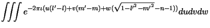
The most straight forward method suggested by Equation 4.5 for
recovering the sky brightness distribution, is to perform a 3D Fourier
transform of ![]() . This requires that the
. This requires that the ![]() axis be also
sampled at the Nyquist rate (Bracewell1986and later eds; Brigham1988and later eds)). For most
observations, it turns out that this is rarely satisfied and doing a
FFT along the third axis would result into severe aliasing.
Therefore, in practice, the Fourier transform on the third axis is
usually performed using the direct Fourier transform (DFT) on the
un-gridded data.
axis be also
sampled at the Nyquist rate (Bracewell1986and later eds; Brigham1988and later eds)). For most
observations, it turns out that this is rarely satisfied and doing a
FFT along the third axis would result into severe aliasing.
Therefore, in practice, the Fourier transform on the third axis is
usually performed using the direct Fourier transform (DFT) on the
un-gridded data.
To perform the 3D FT (FFT along the ![]() and
and ![]() axis and DFT along
the
axis and DFT along
the ![]() axis) one still needs to know the number of planes needed
along the
axis) one still needs to know the number of planes needed
along the ![]() axis. This can be found using the geometry shown in
Fig. 4.2. The size of the synthesized beam along the
axis. This can be found using the geometry shown in
Fig. 4.2. The size of the synthesized beam along the
![]() axis is comparable to that along the other two directions and is
given by
axis is comparable to that along the other two directions and is
given by
![]() where,
where, ![]() is the longest
projected baseline length. The separation between the planes along
is the longest
projected baseline length. The separation between the planes along
![]() should be
should be
![]() . The distance between the tangent
plane and a point separated by
. The distance between the tangent
plane and a point separated by ![]() from the phase center, for
small values of
from the phase center, for
small values of ![]() , is given by
, is given by
![]() . For a field of view of angular size
. For a field of view of angular size ![]() , critical
sampling would be ensured if the number of planes along the
, critical
sampling would be ensured if the number of planes along the ![]() axis,
axis,
![]() , is
, is
Another reason why more than one plane would be required for very high
dynamic range imaging is as follows. Strictly speaking, the only
point which lies in the tangent plane is the point at which the
tangent plane touches the Celestial sphere. All other points in the
image, even close to the phase center, lie slightly below the tangent
plane. Deconvolution of the tangent plane then results into
distortions for the same reason as the distortions due to the
deconvolution of a point source which lies between two pixels in the
2D case (Briggs1995). As in the 2D case, this problem can be
minimized by over sampling the image which, in this case, implies
having more than one plane along the ![]() -axis, even if
Equation 4.6 implies that one plane is sufficient.
-axis, even if
Equation 4.6 implies that one plane is sufficient.
As mentioned above, emission from the phase center and from points close to it, lie approximately in the tangent plane. Polyhedron imaging relies on exploiting this by approximating the Celestial sphere by a number of tangent planes, referred to as facets, as shown in Fig. 4.3. The visibilities are recomputed to shift the phase center to the tangent points of each facet and a small region around each of the tangent points is then mapped using the 2D approximation.
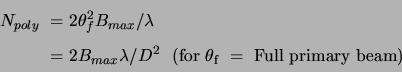
The number of planes required to map an object of size ![]() can be
found simply by requiring that the maximum separation between the
tangent plane and the Celestial sphere be less than
can be
found simply by requiring that the maximum separation between the
tangent plane and the Celestial sphere be less than
![]() ,
the size of the synthesized beam. As shown earlier, this separation
for a point
,
the size of the synthesized beam. As shown earlier, this separation
for a point ![]() degrees away from the tangent point is
degrees away from the tangent point is
![]() . Hence, for critical sampling, the number of planes
required is equal to the solid angle subtended by the sky being mapped
(
. Hence, for critical sampling, the number of planes
required is equal to the solid angle subtended by the sky being mapped
(
![]() ) divided by
) divided by
![]() (
(
![]() )
)
 |
(7.7) |
The polyhedron imaging scheme is implemented in the current version of the AIPS data reduction package and the 3D inversion (and deconvolution) is implemented in the (no longer supported) SDE package developed by T.J. Cornwell et al. Both these schemes, in their full glory, are available in the (recently released) AIPS++ package.
The GMRT 325-MHz data was imaged using the IMAGR task in AIPS.
This program implements the polyhedron algorithm and requires the user
to supply the number of facets to be used and a list of the locations
of the centre of each facet with respect to the image centre and the
size of each facet. This list of facets and their parameters were
computed using the task SETFC in AIPS, typically resulting in a
grid of ![]() facets, each of size
facets, each of size
![]() pixels.
pixels.
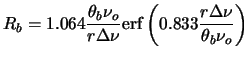
The effect of a finite bandwidth of observation as seen by the
multiplier in the correlator, is to reduce the amplitude of the
visibility by a factor given by
![]() where
where ![]() is the
angular size of the synthesized beam,
is the
angular size of the synthesized beam, ![]() is the center of the
observing band,
is the center of the
observing band, ![]() is location of the point source relative to the
field center and
is location of the point source relative to the
field center and
![]() is the bandwidth of the signal being
correlated.
is the bandwidth of the signal being
correlated.
The distortion in the map due to the finite bandwidth of observation
can be understood as follows. For continuum observations, the
visibility data integrated over the bandwidth
![]() is treated
as if the the observations were made at a single frequency
is treated
as if the the observations were made at a single frequency ![]() -
the central frequency of the band. As a result the
-
the central frequency of the band. As a result the ![]() and
and ![]() co-ordinates and the value of visibilities are correct only for
co-ordinates and the value of visibilities are correct only for
![]() . The true co-ordinates at other frequencies in the band are
related to the recorded co-ordinates as
. The true co-ordinates at other frequencies in the band are
related to the recorded co-ordinates as
| (7.8) |
 |
(7.11) |
The effect of bandwidth smearing can be reduced if the band is split
into frequency channels with smaller channel widths. This effectively
reduces the bandwidth ![]() as seen by the mapping procedure and
while gridding the visibilities,
as seen by the mapping procedure and
while gridding the visibilities, ![]() and
and ![]() can be computed
separately for each channel and assigned to the appropriate uv-cell.
The FX correlator used in GMRT provides up to 128 frequency channels
over the entire bandwidth of observation and the visibilities can be
retained as multi-channel in the mapping process to reduce bandwidth
smearing. Although purely from the point of view of bandwidth
smearing, averaging
can be computed
separately for each channel and assigned to the appropriate uv-cell.
The FX correlator used in GMRT provides up to 128 frequency channels
over the entire bandwidth of observation and the visibilities can be
retained as multi-channel in the mapping process to reduce bandwidth
smearing. Although purely from the point of view of bandwidth
smearing, averaging ![]() channels at 325 MHz would be
acceptable, keeping the visibility database with all the 128 channels
is usually recommended to allow identification and flagging of narrow
bands RFI.
channels at 325 MHz would be
acceptable, keeping the visibility database with all the 128 channels
is usually recommended to allow identification and flagging of narrow
bands RFI.
![\includegraphics[]{Images/Poly.eps}](img592.png)
![$\displaystyle I^d(l,m)=\left[ {\int\limits_0^\infty \vert H_{RF}(\nu)\vert^2 \l...
...u \over {\int\limits_0^\infty \vert H_{RF}(\nu)\vert^2 d\nu}} \right]*DB_o(l,m)$](img611.png)