Appendix D
Computation of antenna based complex gains

(D.1)

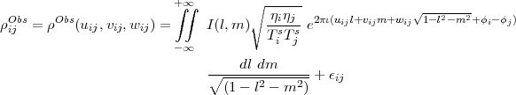
where I(l,m) is the sky surface brightness, η_i is the sensitivity and T_i^s is the system temperature of the antenna i in units of Kelvin/Jy and Kelvin respectively, ϵ_ij is the additive noise on the baseline i-j, and ϕ_i is the antenna based phase of the signal. The rest of the symbols have the usual meaning.

In practice, however, the antenna based amplitude () and phase (ϕ_i) are potentially time varying quantities. This could be due to changes in the ionosphere, temperature variations, ground pick up, antenna blockage, noise pick up by various electronic components, background temperature, etc. Treating the quantities under the square root in the above equation as the antenna dependent amplitude gains, these can be written as complex gains g_i = a_ie^-ιϕ_i where a_i = . For an unresolved source at the phase tracking center, variations in this amplitude will be indistinguishable from a variations in the ratio of η and T^s.

In terms of g_is, we can write Equation D.1 as

(D.2)

where

(D.3)

The use of the word “antenna based gains” for g_is result in confusion for many and needs some clarifications. g_is are called complex “gains” since they multiply with the complex quantity ρ_ij. For an unresolved source, represents the fraction of correlated signal and arg(g_i) represents the phase of the correlated part of the signal from the antenna with respect to the phase reference (usually the reference antenna). It is in this sense that it is referred to as “antenna based” gains. However, as defined here, they include T^s which in turn includes the sky background temperature. They are therefore a function of direction in the sky. However, here we assume that the angular scale over which g_is vary is larger than the antenna primary beam (isoplanatic case).

For an unresolved source at the phase tracking center, all terms in the exponent of ρ_ij^∘ are exactly zero. ρ_ij^∘ in this case would be proportional to the flux density of the source.

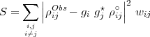
Assuming that the antenna dependent complex gains are independent, with a gaussian probability density function (this implies that the real and imaginary parts are independently gaussian random processes), one can estimate g_is by minimizing, with respect to g_is, the function S given by

(D.4)

where w_ij = 1∕σ_ij², σ_ij being the variance on the measurement of ρ_ij^Obs

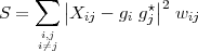
Dividing the above equation by ρ_ij^∘ (the source model, which is presumed to be known – it is trivially known for an unresolved source), and writing ρ_ij^Obs∕ρ_ij^∘ = X_ij, we get

(D.5)

If ρ_ij^∘ represents the structure of the source accurately, X_ij will have no source dependent terms and is purely a product of the two antenna dependent complex gains.

Expanding Equation D.5, we get

(D.6)

Evaluation ∂S _ ∂g_i^⋆ and equating it to zero ¹ , we get

(D.7)

or

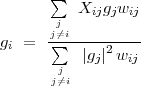(D.8)

This can also be derived by equating the partial derivatives of S with respect to real and imaginary parts of g_i as shown in Section D.3.

Since the antenna dependent complex gains also appear on the right-hand side of Equation D.8, it has to be solved iteratively starting with some initial guess for g_js or initializing them all to 1.

Equation D.8 can be written in the iterative form as:

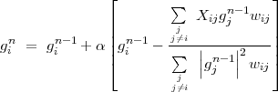(D.9)

where n is the iteration number and 0 < α < 1. Convergence would be defined by the constraint

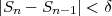(D.10)

(the change in S from one iteration to another) where δ is the tolerance limit.

D.1 Interpretation of the equation

Equation D.8 offers itself for some intuitive understanding in the following way.

X_ij is a product of two complex numbers, namely g_i and g_j^⋆, which we wish to determine. X_ij is itself derived from the measured quantity V _ij^Obs. Numerically speaking, each term in the summation of the numerator of Equation D.8 will involve g_i (via X_ij) and the multiplication of X_ij with g_jw_ij would give g_i an effective weight of ²w_ij. Since the denominator is the sum of this effective weight, the right-hand side of Equation D.8 can be interpreted as the weighted average of g_i over all correlations with antenna i.

In the very first iteration, when g_j = (1,0), the normalization would be incorrect since the numeric value of g_j, as it appears inside X_ij would be different from that used in the denominator of Equation D.8. However, as the estimates of g_js improve with iterations, the equation would progressively approach a true weighted average equation. The speed of convergence will depend upon the value of α and the convergence would be defined by the constraint in Equation D.10. In the ideal case when the true value of all g_is is known, right hand side of Equation D.8 also reduces of g_i.

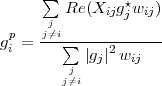
Estimating g_i for an antenna, by averaging over the measurements from all baselines in which it participates (for a unresolved source) makes sense since for an N element array, g_i would be present in N-1 measurements (all the _j=1,N;j≠i) and the best estimate of g_i would be the weighted average of all these measurements. Proper weight for g_i, buried in each of the products X_ij, can be found heuristically as follows. g_i, estimated from the measurements of a given baseline, must obviously be weighted by the signal-to-noise ratio on that baseline. This is w_ij in the above equations. It must also be weighted by the amplitude gain of the other antenna making the baseline, namely g_j, to account for variation in antenna sensitivities and T^s. The total weight for g_i would then be ²w_ij, the sum of which appears in the denominator of Equation D.8. Knowing that ideally X_ij = g_ig_j^⋆, each of the _j=1,N must be multiplied by g_jw_ij (to apply the the above mentioned weights to g_i), before being summed for all values of j and normalized by the sum of weights to form the weighted average of g_i. One thus arrives at Equation D.8 using these heuristic arguments.

D.2 Estimation of the system temperature (T^s)

For an unresolved source of known brightness I, in the limit T^a ≪ T^s, ρ_ij^∘ = I and Equation D.1 can be written as

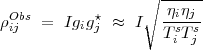(D.11)

where η_i = A_e∕2k_b, A_e is the effective area of the dish, k_b is the Boltzman’s constant and

(D.12)

Hence, knowing η_i, T_i^s can be estimated from the amplitude of the antenna dependent complex gains.

All contributions to ρ_ij^Obs, which cannot be factored into antenna dependent gains, will result in the reduction of . η remaining constant, this will be indistinguishable from an increase in the effective system temperature. Since majority of later processing of interferometry data for mapping (primary calibration, bandpass calibration, SelfCal, etc.) is done by treating the visibility as a product of two antenna based numbers, this is the effective system temperature which will determine the noise in the final map (though, as a final step in the mapping process, baseline based calibration can possibly improve the noise in the map).

In the normal case of no significant baseline based terms (ϵ_ij) in X_ij, the system temperature as measured by the above method will be equivalent to any other determination of T_i^s.

T^s can also be determined by recording interferometric data for a strong point source with and without an independent noise source of known temperature at each antenna. In this case

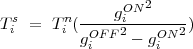(D.13)

where g_i^ON and g_i^OFF are the antenna dependent gains with and without the noise source of temperature Tⁿ. Note that η_i does not enter this equation. Also, Tⁿ should be such that ≥ 0.1 to ensure that the correlated signal is measured with sufficient signal-to-noise ratio. For example, for P-band, a calibrator with P-band flux density > 5 Jy must be used.

D.3 Derivation of g_i using real and imaginary parts

g_is are complex functions. One can therefore write S in terms of g_i^I and g_i^p, the real and imaginary parts of g_i and minimize with respect to g_i^I and g_i^p separately. It is shown here that the complex arithmetic achieves exactly this and the results are same as that given by complex calculus. The superscripts I and R in the following are used to represent the real and imaginary parts of complex quantities.

Expanding Equation D.5, ignoring w_ijs and writing it in terms of real and imaginary parts we get

(D.14)

where

(D.15)

Taking partial derivative of S with respect to g_i^p and reintroducing w_ij, we get

(D.16)

Therefore,

(D.17)

Equating ∂S _ ∂g_i^p to zero, we get

(D.18)

Similarly

(D.19)

Therefore the equivalent imaginary part of Equation D.18 is

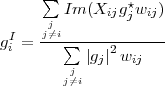(D.20)

writing g_i = g_i^p + ιg_i^I and substituting for g_i^p and g_i^I from Equation D.18 and D.20 respectively, we get

(D.21)

This is same as Equation D.8, which was arrived at by evaluating a complex derivative of Equation D.5 as ∂S∕∂g_i^⋆, treating g_i and g_I^⋆ as independent variables. Evaluating ∂S ∂g_i = 0 would give the complex conjugate of Equation D.21. Hence, ∂S∕∂g_i gives no independent information not present in ∂S∕∂g_i^⋆.