Thus, clearly, Route-b is the most appropriate.
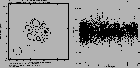
Therefore, solution for the gains of the Central square and the
nearest arm-antennas W01, W02, E02 and S01 were found
using the map obtained using baselines up to ![]() (see the
panel 3 of Fig. 2). The data so calibrated was imaged and the
resulting image was also self-calibrated once. This image was then
used as the image model in the next step. If this step was
successful, then this image (Fig. 4) should produce a better
model for the observed visibilities corrected for the antenna based
offsets (
(see the
panel 3 of Fig. 2). The data so calibrated was imaged and the
resulting image was also self-calibrated once. This image was then
used as the image model in the next step. If this step was
successful, then this image (Fig. 4) should produce a better
model for the observed visibilities corrected for the antenna based
offsets (
![]() ). To check this we
Fourier inverted the map to obtain the model visibilities
(i.e.
). To check this we
Fourier inverted the map to obtain the model visibilities
(i.e.
![]() ). If the model matches the data then
). If the model matches the data then
![]() /
/
![]() should be close to unity, which is
indeed true (see panel 2 of Fig. 4 for the normalized plot).
should be close to unity, which is
indeed true (see panel 2 of Fig. 4 for the normalized plot).
 |
 |
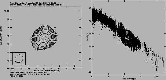
In the next iteration, UVRAN was increased to ![]() and
antennas E03, S02, S03 and W03 were also included. Input
image model was the image from previous iteration (see
Fig. 4). (see Fig. 5 for the map and the normalized
plot. Map was also Self-calibrated).
and
antennas E03, S02, S03 and W03 were also included. Input
image model was the image from previous iteration (see
Fig. 4). (see Fig. 5 for the map and the normalized
plot. Map was also Self-calibrated).
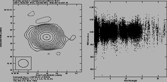
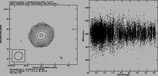
In the final iteration, we also included E04, E05, E06, W04, W05,
S04, W06 and S06 (i.e. the entire array). Again, as before,
the input model image was the image from the previous iteration (the
image in Fig. 6) and UVRAN increased to ![]() .
Obviously, the gains so obtained should be applicable to all the
visibilities (i.e. UVRAN=0). Panel 2 in the Fig. 6
shows the calibrated amplitude for the whole data. Again, if the
method was successful, then
.
Obviously, the gains so obtained should be applicable to all the
visibilities (i.e. UVRAN=0). Panel 2 in the Fig. 6
shows the calibrated amplitude for the whole data. Again, if the
method was successful, then
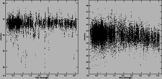
![]() /
/
![]() should be
close to unity. Fig. 7 shows that this is indeed true.
Fig. 7 also shows the final image at full GMRT resolution.
should be
close to unity. Fig. 7 shows that this is indeed true.
Fig. 7 also shows the final image at full GMRT resolution.