This note is under construction ! We are verifying correctness....
This memo attempts to generate expression(s) for the steady-state memory footprint of the CASA imager. By ``steady state'', we mean the combined memory required for one major- and one minor-cycle. The expressions for the total memory are also factored into seperate terms for major- and minor-cycle memory footprints. Note that while there is some analysis, this memo is primarily focused on describing the current memory footprint and not for describing the why of the footprint for various algorithms.
If you are not interested in the details, you can directly read Eqs. 4.4, 4.8, 4.15 and 4.16 for the memory footprint for classical Clean, MS-Clean, MS-MFS Clean and Mosaic Clean respectively. Memory footprint in units of number of N-pixel sized images for typical values of the associated parameters for classical Clean, MS Clean and MS-MFS Clean are given in Tables 4.1, 4.2 and 4.3 respectively.
The equations are parametrized by the size of the user-defined image
(
![]() ), number of visibility plane polarizations used
(
), number of visibility plane polarizations used
(![]() ) to generate the user-defined number of image-plane
polarization planes (
) to generate the user-defined number of image-plane
polarization planes (![]() ), number of user-defined scales
(
), number of user-defined scales
(![]() ) and Taylor-terms (
) and Taylor-terms (![]() ) for MS Clean, and MS-MFS Clean.
Since the overheads are different for different classes of
algorithms, the equations are also separated in three different
classes:
) for MS Clean, and MS-MFS Clean.
Since the overheads are different for different classes of
algorithms, the equations are also separated in three different
classes:
The constant overhead which is constant across all classes of
algorithms consists of 3 scratch images, one mask-image and one
complex image, each with ![]() number of planes
number of planes
The computing cost of gridding/de-gridding scales with the number of visibility points and the convolution function support area. For large data-sets (which do not fit in the computer RAM), the run-time cost is dominated by data I/O.
To minimize this data I/O, CASA imager holds separate complex
grids for forward and reverse transforms. Each pixel of one of these
grids consumes single-precision complex storage, while the other has
double precision complex storage. Each has ![]() number of
polarization planes. The total storage for these grids is therefore
number of
polarization planes. The total storage for these grids is therefore
For the image-plane operations of Clean, we hold one FP-image each to
represent the residual image ![]() , the PSF
, the PSF ![]() and the model
image
and the model
image ![]() . Each has
. Each has ![]() number of polarization planes.
Together the amount of memory they use is
number of polarization planes.
Together the amount of memory they use is
The total memory foot print for single pointing non-MS, non-MFS-MFS
Clean is the sum of Eqs. 4.1, 4.2 and 4.3.
The major-cycle memory footprint is given by the first two terms and the minor-cycle memory footprint is given by the last term in the following expression:
| (4.5) |
| (4.6) |
In addition to the above, MS-Clean has an overhead of holding one
image per scale
![]() , one mask-image per scale
, one mask-image per scale
![]() and a scratch image
and a scratch image
![]() . All these have
. All these have ![]() number of polarization planes. Further, complex images
number of polarization planes. Further, complex images
![]() per scale,
per scale, ![]() and
and ![]() are also allocated.
The MS-Clean code additionally also allocated the
are also allocated.
The MS-Clean code additionally also allocated the
![]() image with
image with ![]() polarization planes. The total memory
footprint for this is:
polarization planes. The total memory
footprint for this is:
![$\displaystyle I^{dirtycopy} + \left[ \frac{N_S(N_S+1)}{2} \right] I^{PSF}_{MS} ...
...eMask} + N_s I^{dirty*scale} + I^{mask}+
N_s I^{scaleXFR} + I^{XFR} + I^{cWork}$](img49.png) |
|||
![$\displaystyle N + \left[ \frac{N_S(N_S+1)}{2}N \right] + N_s \left[N+N+N\right]+N
+ 2\times \frac{N_s N}{2} + 2\times \frac{N}{2} + 2\times N$](img50.png) |
|||
![$\displaystyle \frac{N}{2}\left[N^2_s + 9 N_s + 10 \right]$](img51.png) |
(4.7) |
In addition, storage for residual images per scale is also required.
For the PSF images, the PSF corresponding to the cross-terms between
scales is also computed. All these also have ![]() number of
polarization planes. The total memory required for MS-Clean is therefore
number of
polarization planes. The total memory required for MS-Clean is therefore
The major-cycle memory footprint is given by the first two terms and the minor-cycle memory footprint is given by the last term in the following expression:
 |
(4.9) |
|
MS-MFS needs to account for the cross terms between scales
and Taylor-terms. To account for the coupling between scales and
Taylor terms, the number of images required for the MS-MFS Clean is
| (4.10) |
Additionally, MS-MFS also has the following storage overheads. Note
that are
![]() ,
, ![]() ,
,
![]() , and
, and
![]() are
half-complex images.
are
half-complex images.
| (4.11) | |||
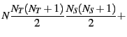 |
|||
 |
(4.12) | ||
 |
(4.13) |
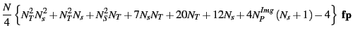
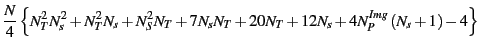
The total memory footprint for the single pointing MS-MFS Clean
therefore is
|
For mosaic imaging, an extra single-precision complex grid is
allocated. Depending on the algorithm used (classical,
MS-Only, MS-MFS), the memory footprint is
![$\displaystyle 6 N N^{Vis}_P + 10NN^{Img}+\frac{N}{2}\left[N^2_s + 9N_s + 10\right]$](img54.png)
![$\displaystyle \frac{N}{2}\left[12N^{Vis}_P+20N^{Img}_P+N^2_s+9N_s+10\right] {\tt\bf
fp}$](img55.png)