2.3 Summaries, displays, reports

2.3.1 Flag summaries

Screenshot of runtime flag

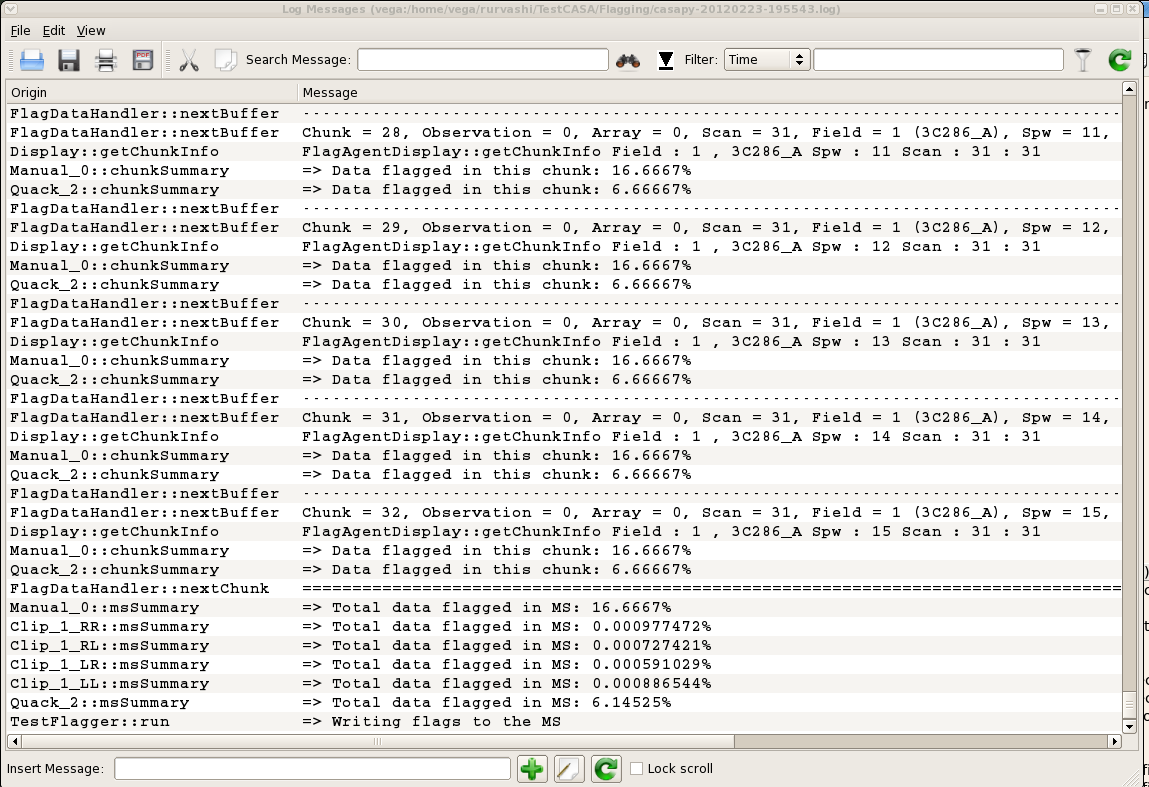
Figure 9: Example of runtime logger summary of flag counts per agent

2.3.2 Flag Reports/Views

Here are some examples of flag report displays on two datasets.

1. Percentage of data flagged vs frequency : To assess how much usable data is present in each spectral-window, for later processing, and imaging sensitivity-estimates.
2. Percentage of data flagged vs antenna-position : To assess whether the RFI is restricted to only some antennas and therefore may be local.
3. Percentage of data flagged vs baseline-length : To assess expected sensitivities for different spatial scales, since local RFI correlates better on shorter baselines than longer ones.

2.3.3 Data Display + action='calculate'

In order to visualize some of the RFI present in the data, and to verify if flagging commands are having the desired effect, there is an option to visualize the data and flags at run-time, and navigate between baselines in the current chunk, as well as in the forward-direction across scans and spws.

The intended usage of the display is to run the flagger on small subsets of the data (sub-selections) with action='calculate', and display='data', and inspect the flagging results. An option to quit at any stage allows the user to change input parameters and try again until the desired flagging results are obtained. Then, the display can be turned off, action set to 'apply', and the program run again on a larger section of the data.