2.1 Single flag mode (flagdata)

All the following flagging modes operate on user-specified subsets of the data. The dataset is iterated-through in chunks consisting of one field, one spw, and a user-defined timerange (default is one scan). Modes that read visibilities also respond to some simple expressions that are applied to the visibilities, before they are considered for flagging (for example, $ABS\_RR,LL, ABS\_I, REAL\_V, ABS\_ALL$ ).

2.1.1 Manual Flag/Unflag

Selection-based flagging and unflagging can be done via the MSSelection syntax. This flagging mode is meant for marking subsets of the data that are known to be unfit for calibration or imaging. Some examples are online flags from the data-recording system, known frequency ranges with strong RFI, etc. It is also possible to use the parameter 'autocorr' to flag only auto-correlations in the MS.

2.1.2 Quack

Data at scan edges can sometimes be unusable for some antennas or baselines (for example, if some antennas take longer than others to slew to a new target, but the signal correlation and recording starts before all antennas are ready), and it is often useful to flag these edges.The 'quack' mode allows the user to specify time-ranges from the beginning and/or end of all selected scans.

2.1.3 Elevation

Data taken when the antennas are pointed at low elevations can sometimes be unusable and require flagging. Reasons for flagging data at low elevations include increased shadowing between antennas, increased sensitivity to RFI from the horizon, elevation-dependent antenna-gain variations, corrupted spectra due to looking through a longer path-length through the atmosphere, etc. At high elevations, one problem could be increased pointing errors when an Alt-Az antenna tracks a source near the Zenith. The 'elevation' mode allows the user to specify elevation-ranges to be flagged, for the selected data.

2.1.4 Clip

Strong outliers can be flagged using a simple threshold (range). If a valid data range is known $a-priori$ , clipping can be done as the first step before basic calibration or other editing. The 'clip' mode allows the user to specify a range, and clip all values either within or outside the range. Values are defined as expressions that involve data columns and correlation-selections (for example, ABS_I or REAL_RR,LL, etc). NaNs and Infs are always included in the clipping. By default, if no range for clipping is given, it will flag only NaNs and Infs. Optionally, exact zeros can flagged using the clipzeros parameter. Early EVLA data-sets occasionally have exact zeros in parts of the data where the backend-system is overloaded, and NaNs and Infs have sometimes been reported when data is converted between packages and formats.

2.1.5 Shadow

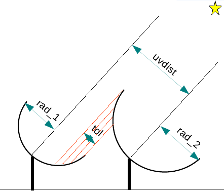
Shadow flags are computed by considering the positions and diameters of a list of antennas along with the target direction at each timestep. All antennas present in the ANTENNA subtable of the MS as well as any other positions and diameters supplied via an external file are considered for shadow-flag calculations.

Shadow flags are computed as follows (for every timestep):

1. Calculate or read the $u,v,w$ values (in meters) for all possible antenna-pairs, using the phase-reference center of the observation to define the pointing-direction. The values of $u,v,w$ are re-used when already present in the MS, and calculated only for baselines without visibilities in the current timestep (to account for antennas that did not produce data for that timestep, but were still physically present and creating shadows).

2. For each possible antenna pair, use the value of $w$ to determine which antenna is behind and which is in front ( $w<0$ : antenna 1 is behine antenna 2 ).

3. Mark the 'behind' antenna for flagging if $\sqrt{u^2+v^2} < r_1 + r_2 - tol$ . Here, $r_1,r_2$ are the radii of the two antennas, and $tol$ is the amount (in meters) of allowed shadowing before being marked for flagging.

Figure 3: This figure shows the geometry used to compute shadowed antennas.

Note : The use of the phase-reference center as the pointing-direction for all antennas, is accurate in most cases, but will be approximate during on-the-fly mosaicing. However, since it is unlikely that an on-the-fly mosaic will be done with only one phase-reference center on a large-enough field-of-view for shadow-flag differences to become significant.

Note : Antennas that are not part of the MS ANTENNA subtable can be included in the calculation of shadow flags by specifying a list of positions and diameters in an external file. Note however that the calculations will not account for the fact that antennas not part of the observation, but still physically present on the ground, may not be pointing in the same direction as all the others (as is assumed in the calculations). If desired, the antenna diameters in the external file could be adjusted accordingly.

Example :

name=VLA1
diameter=25.0
Position=[-1601144.96146, -5041998.01971, 3554864.76811]

name=VLA2
diameter=25.0
position=[-1601105.76646, -5042022.39178, 3554847.24515]

A helper-function has been provided to construct this list from an MS (possibly a different dataset) that contains the required information in its ANTENNA subtable.

import flaghelper;
antlist =  flaghelper.extractAntennaInfo (
            msname='shadowtest.ms',
            antnamelist=['VLA1','VLA2','VLA9','VLA10'] );
flaghelper.writeAntennaList('antlist.txt',antlist);

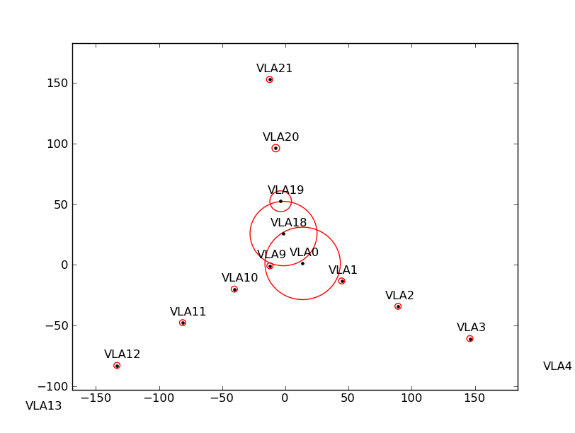
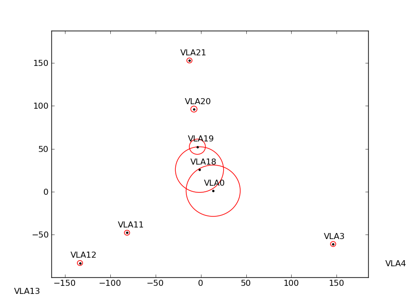
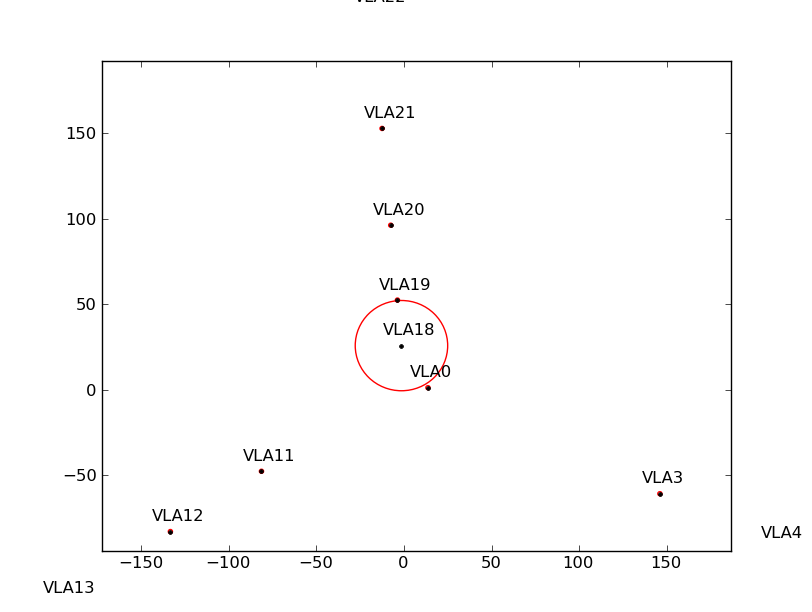
Figure shows the flagging results from a simulated observation that spans a large elevation range. Antennas near the center of the array are shadowed more than the others (left plot). If some antennas are split-out of the dataset, the ANTENNA subtable will have fewer antennas, and the shadow flags will change (middle plot). However, by specifying the positions and diameters of the missing antennas via the external file, the correct shadow flags are recovered (right plot).

Figure 4: This figure shows fractions of data flagged per antenna, for three different use-cases. The size of the circle is proportional to the fraction of data flagged. (LEFT) : Shadow-Flags with all antennas present in the MS, (MIDDLE) : Shadow-Flags with four antennas (and their baselines) deleted from the MS, (RIGHT) : Shadow-Flags from the MS with the missing antennas, but with the positions and diameters of the missing antennas specified via an external text file. The flags produced are the same as when all antennas are present in the MS.

2.1.6 TFCrop

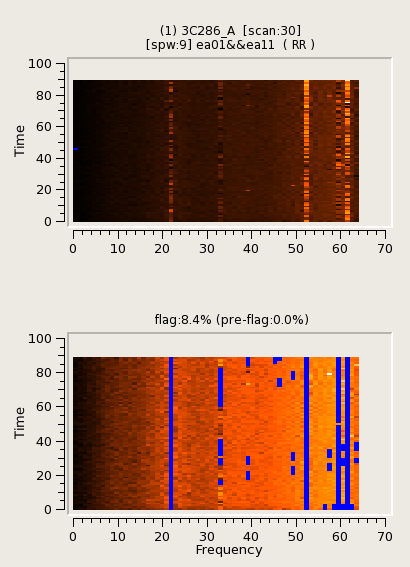
TFCrop is an autoflag algorithm that detects outliers on the 2D time-frequency plane, and can operate on un-calibrated data (non bandpass-corrected).

The original implementation of this algorithm is described in NCRA Technical Report 202 (Oct 2003)

The algorithm iterates through the data in chunks of time. For each chunk, the result of user-specified visibility-expressions are organized as 2D time-frequency planes, one for each baseline and correlation-expression result, and the following steps are performed.

1. Calculate a bandshape template : Average the data across time, to construct an average bandpass. Construct an estimate of a clean bandpass (without RFI) via a robust piece-wise polynomial fit to the average bandpass shape.

   Note : A robust fit is computed in upto 5 iterations. It begins with a straight line fit across the full range, and gradually increases to 'maxnpieces' number of pieces with third-order polynomials in each piece. At each iteration, the stddev between the data and the fit is computed, values beyond N-stddev are flagged, and the fit and stddev are re-calculated with the remaining points. This stddev calculation is adaptive, and converges to a value that reflects only the data and no RFI. At each iteration, the same relative threshold is applied to detect flags, and this results in a varying set of flagging thresholds, that allows deep flagging only when the fit represents the true data best. Iterations stop when the stddev changes by less than 10%, or when 5 iterations are completed.

   The resulting clean bandpass is a fit across the base of RFI spikes.

2. Divide out this clean bandpass function from all timesteps in the current chunk. Now, any data points that deviate from a mean of 1 can be considered RFI. This step helps to separate narrow-band RFI spikes from a smooth but varying bandpass, in situations where a simple range-based clipping will flag good sections of the bandpass.

3. Perform iterative flagging (robust flagging) of points deviating from a value of 1.

   Flagging is done in upto 5 iterations. In each iteration, for every timestep, calculate the stddev of the bandpass-flattened data, flag all points further than N times stddev from the fit, and recalculate the stddev. At each iteration, the same relative threshold is applied to detect flags. Optionally, use sliding-window based statistics to calculate additional flags.

4. Repeat steps 1 and 3, but in the other direction (i.e. average the data across frequency, calculate a piece-wise polynomial fit to the average time-series, and find flags based on deviations w.r.to this fit.)

The default parameters of the tfcrop implementation are optimized for strong narrow-band RFI. With broad-band RFI, the piece-wise polynomial can sometimes model it as part of the band-shape, and therefore not detect it as RFI. In this case, reducing the maximum number of pieces in the polynomial can help. This algorithm usually has trouble with noisy RFI that is also extended in time of frequency, and additional statistics-based flagging is recommended (via the 'usewindowstats' parameter). It is often required to set up parameters separately for each spectral-window.

If frequency ranges of known astronomical spectral lines are known $a-priori$ , they can be protected from automatic flagging by de-selecting those frequency-ranges via the 'spw' data-selection parameter.

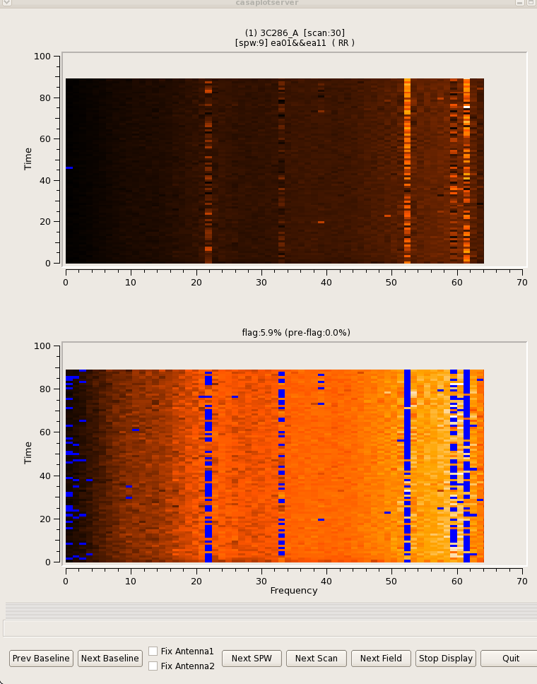
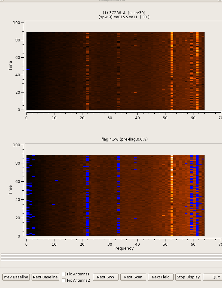
Below are some examples that demonstrate what the algorithm does with different types of RFI.

Figure 5: LEFT : This screenshot represents a run where 'tfcrop' was run on a spw='9' with mainly narrow-band RFI. RIGHT : An example of protecting a spectral line (in this case, demonstrated on an RFI spike) by setting the spw-selection to spw='0:0 45;53 63'. In both figures, the top row indicates the data before flagging, and the bottom row after flagging.

2.1.7 RFlag

RFlag is an autoflag algorithm based on a sliding window statistical filter (E.Greisen, AIPS, 2011).

The RFlag algorithm was originally developed by Eric Greisen in AIPS (31DEC11).
AIPS documentation : Subsection E.5 of the AIPS cookbook (Appendix E : Special Considerations for EVLA data calibration and imaging in AIPS)

In RFlag, the data is iterated-through in chunks of time, statistics are accumulated across time-chunks, thresholds are calculated at the end, and applied during a second pass through the dataset.

The CASA implementation also optionally allows a single-pass operation where statistics and thresholds are computed and also used for flagging, within each time-chunk (defined by 'ntime' and 'combinescans').

For each chunk, calculate local statistics, and apply flags based on user supplied (or auto-calculated) thresholds.

1. Time analysis (for each channel)
   1. Calculate local rms of real and imag visibilities, within a sliding time window
   2. Calculate the median rms across time windows, deviations of local rms from this median, and the median deviation
   3. Flag if local rms is larger than timedevscale x (medianRMS + medianDev)
2. Spectral analysis (for each time)
   1. Calculate avg of real and imag visibilities and their rms across channels
   2. Calculate the deviation of each channel from this avg, and the median-deviation
   3. Flag if deviation is larger than freqdevscale x medianDev

Reports and plots are generated from rflag (when writeflags=False), to display the mean deviations for each channel, as well as the mean variance of local statistics from this median deviation (local statistics are computed in a sliding-window).

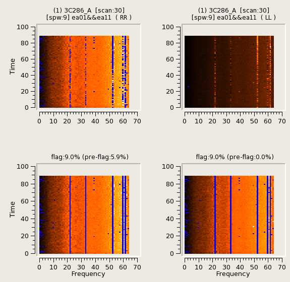
Below are some examples.

1. Calculate thresholds automatically per scan, and use them to find flags. Specify scale-factor for time-analysis thresholds, use default for frequency.

      flagdata('my.ms', mode='rflag',spw='9',timedevscale=4.0,writeflags=True)
   

2. Supply noise-estimates to be used with default scale-factors.

      flagdata(vis='my.ms', mode='rflag', spw='9', timedev=0.1, freqdev=0.5, writeflags=True);
   

3. Two-passes. This replicates the usage pattern in AIPS.

   - The first pass saves commands in an output text files, with auto-calculated thresholds. Thresholds are returned from rflag only when writeflags=False (calc-only mode). The user can edit this file before doing the second pass, but the python-dictionary structure must be preserved.

   - The second pass applies these commands (writeflags=True).

     flagdata(vis='my.ms', mode='rflag', spw='9,10',                                               timedev='tdevfile.txt', freqdev='fdevfile.txt', writeflags=False);
     flagdata(vis='my.ms', mode='rflag', spw='9,10', 
               timedev='tdevfile.txt', freqdev='fdevfile.txt', writeflags=True);
   

Figure 6: Example of rflag on narrow-band RFI

2.1.8 Extend

Flags can be extended along various axes (within one spw, field, and time-chunk). Autoflag algorithms on their own often leave out pieces of RFI-affected data, in-between flagged points, and flag extensions are often useful. Data points can be flagged if more than half of the surrounding points are already flagged. If a timerange or frequency-range is more than (for example) 50% flagged, the entire range can be flagged. Flags can be extended across correlations, in cases where the RFI-signal-to-noise ratio is higher in some correlations where it is easier to detect than in other correlations.

Figure 7: This screenshot represents a run where 'tfcrop' was run only on 'ABS_RR' (top row) and followed by an extension along time and correlations (bottom row).