1.1 C++ Infrastructure

1.1.1 Framework

1.1.1.1 Main Classes

1. AgentFlagger: The top-level AgentFlagger class that connects all of the following together, and defines the C++ user-interface for the agentflagger. This is the class used by the tool layer.

2. FlagDataHandler : A top level class defining the data handling interface for the flagging module.

3. The FlagAgentBase base class defines the behaviour of all flagging agents and contains agent-level data-selection, etc. The main functions to be implemented by derived classes are setAgentParameters(), preProcessBuffer(), computeAntennaPairFlags() or computeRowFlags(), getReport() .

   List of available Flag Agents :

   1. FlagAgentManual : Flag/Unflag based on data-selections. The only processing done by this agent is to set the flags for all data it sees to True if the operation is to flag, and to False to unflag. A boolean parameter apply determines whether to flag (apply=True) or unflag (apply=False). By default it is set to True.

   2. FlagAgentQuack : Flag time-ranges at the beginning and/or end of scans. Uses the YYY iteration-mode.

   3. FlagAgentElevation : Flag time-ranges based on source elevation. Uses the YYY iteration-mode.

   4. FlagAgentShadow : For each timestep, flag antennas that are shadowed by any other antenna. Antennas to be flagged are chosen and marked in the preProcess() stage. Rows are flagged in computeRow(), and this agent uses the YYY iteration-mode.

   5. FlagAgentExtend : Read and extend flags along specified axes, within the current chunk. Uses the YYY iteration-mode.

   6. FlagAgentClip : Flag based on a clip threshold and visExpression. Find and flag NaNs and Infs. Uses the YYY iteration-mode.

   7. FlagAgentTimeFreqCrop : The TFCrop algorithm is run per baseline, via FlagAgentTimeFreqCrop::computeAntennaPairFlags()

   8. FlagAgentRFlag : The RFlag algorithm. Implements multiple passes through each chunk via the passIntermediate() and passFinal() mechanism.

   9. FlagAgentSummary : Flag counts are accumulated in computeRow() and packaged into a Record in getResult().

   10. FlagAgentDisplay : Visibilities are read and displayed from computeAntennaPair(). Navigation-buttons control the order in which the framework iterates through baselines.

4. The FlagReport class allows each flag agent to build and return information (summary counts, reports as plots, etc) to the user (and/or) to the display agent for end-of-MS reports.

1.1.2 Control Flow

1.1.3 Performance Optimizations

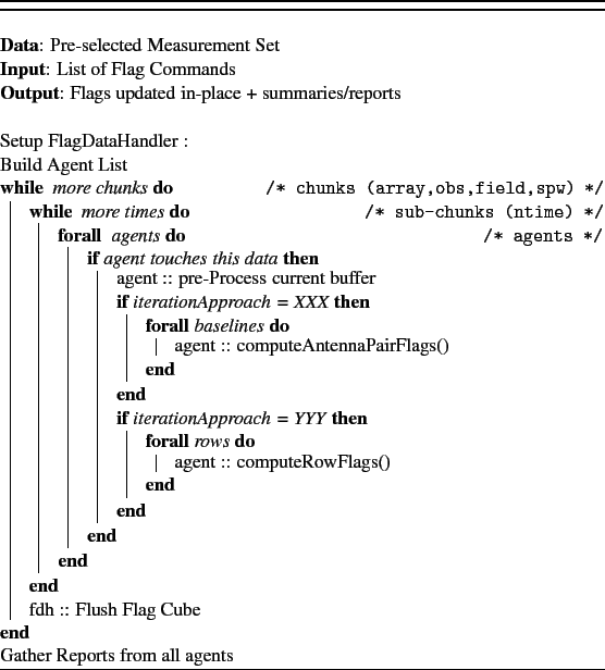
There are several performance-optimization choices that can be made. Some of these are under the users control, and some have automated heuristics.

1.1.3.1 List mode

It helps to combine multiple flag commands into a single run ONLY if most of the commands require the same data to be read.

The goal is to read data once, apply multiple flag commands, and write flags once.

1. Manual-flag commands read only meta-data.
2. Shadow, elevation read meta-data + processing to calculate uvw, azel.
3. Clip reads visibilities.
4. tfcrop and rflag read visibilities and flags
5. Extend, summary read flags

1.1.3.2 Data pre-selection

If only a subset of the Measurement Set is to be traversed for flag-calculation, it helps to pre-select and iterate through only that section of the MS. When multiple flag commands are supplied, with different data-selections, this pre-selection is calculated as a loose union of all input selection parameters (currently a list of all unique spectral-windows and field-ids).

This is done automatically at the task level, and is in the control of the user at the tool level (via af.selectdata().

Note that there is a second level of selection per agent (command) that ensures that each agent (command) sees only its correct subset of the data. The above pre-selection is purely for optimization reasons to prevent the infrastructure from stepping through and rejecting untouched parts of the data (even though the meta-data reads requires for the checks per chunk are minimal).

1.1.3.3 Asynchronous I/O

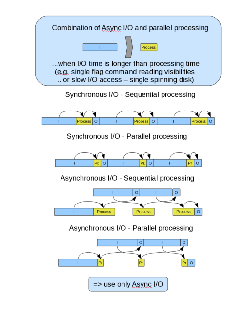
Asynchronous I/O is a data-access optimization that applies when iterating through the dataset in chunks. It uses multi-threading to pre-read the next chunk of data from disk while the current chunk is being processed.

The user has the option of enabling asynchronous I/O by setting the following variables in the .casarc file.

VisibilityIterator.async.enabled: true     # if present and set to false then async i/o will work
VisibilityIterator.async.nBuffers: 2       # the default value is two
VisibilityIterator.async.logFile: stderr   # Send async i/o debug log messages to this file
                                           # if not present or file is invalid then no logging occurs
VisibilityIterator.async.logLevel: 2       # Level of log messages to output (two is good, too); defaults to 1

FlagDataHandler.asyncio: true                # True : enable async-IO for the flagger (clip,tfcrop,rflag)
FlagDataHandler.slurp: true                  # True : enable ??
FlagAgent.background: true                   # True : enable threading mode

Asynchronous I/O helps ONLY when data I/O dominates the total cost. For our current list of agents/algorithms, this helps only for agents that read visibilities. Therefore asynchronous I/O is activated only if clip or tfcrop or rflag are present in the flag-command list.

1.1.3.4 Agent parallelization

Parallel execution of flagging agents helps when processing dominates the runtime, but there are several factors that will affect performance. Parallelization by agent is helpful only if there is a list of agents of similar type, and the number of agents is less than the number of available cores. Parallelization by data-partitioning (chunks of baselines, for example) is useful if all agents touch all baselines and do not require communication across baselines).

Agent-level parallelization is currently disabled, but as part of CAS-3861, heuristics will be implemented internally, and then documented here.

1.1.3.5 Interaction between Async IO and Agent parallelization

Figures 1 symbolically shows how async-IO and agent parallelization would scale when IO dominates, vs when processing dominates.

Figure 1: Explanation...

1.1.4 Timing Tests

Data :

Continuum : few fat channels.
SpectralLine : many thin channels.

SinglePointing : contiguous scans on the same field
Mosaic : each scan is a different fields.

1. L-band continuum , Single Pointing --- need to decide dataset (probably G55.7+3.4_1s.ms)
2. L-band spectral-line , Mosaic --- need to pick dataset

1.1.4.1 Comparison between modes

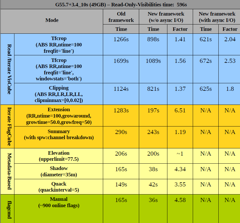
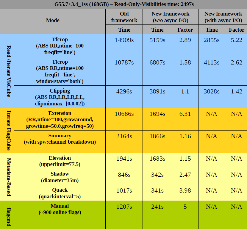
Figure 2: These tables show timing comparisons between various modes, for two EVLA continuum datasets. Parameters of the datasets are...

1.1.4.2 Break-down of timings

: if possible, with and without async-IO.

1. Only-reading-visibilities
2. Only-reading flags
3. Only-writing flags
4. (pls ignore if this makes no sense.) Only-iterating through the visbuffers without reading/writing anything (i.e. to see if much time is saved by the loose union).

1.1.4.3 Comparison between data-shapes and iteration patterns

Two types of datasets : wideband continuum single-pointing, spectral-line mosaic