3.4 Comparison of RFI with 1s vs 10s integrations

In order to reduce dataset sizes, data can be averaged during the observation. However, with integration-times of anything larger than few seconds, there is the risk of smearing out the RFI and losing a larger fraction of the data to RFI.

The following is the result of a few autoflag tests on an L-Band D-config 7-hour dataset (G55.7+3.4), for which we have a version with 1sec integrations,a 10s averaged version (with and without pre-applying online flags).

Figures 13 and 14 show the percentage of data flagged per frequency-channel for the 1sec and 10sec datasets respectively, showing a few% less data flagged in the 10sec dataset. Figures 15 and 16 show the percentage flagged per antenna and scan (each scan is 1.5 minutes long), and show a difference of about 1% in the amount of data flagged by 'rflag', indicating that there is no practical loss of data due to smearing out of the RFI during the 1sec-to-10sec averaging. Figure 17 is the result of applying online flags on the 1-sec data before averaging to 10-sec and running rflag. Comparing with the previous plots, this saves about 1% to 2% of the flagged data.

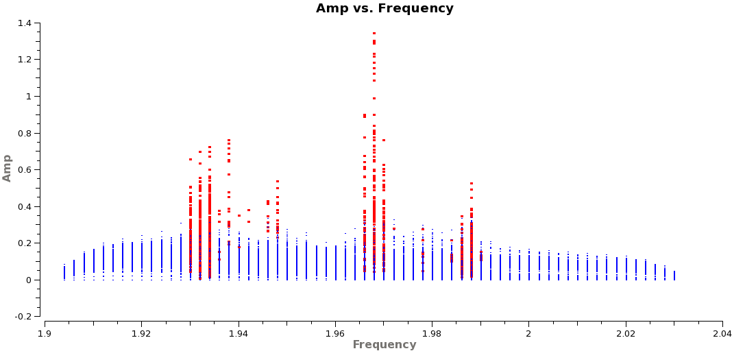
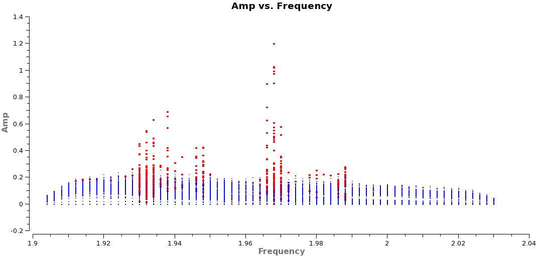
Figure 18 shows plots of the un-calibrated data for the first two cases (1sec and 10sec), to demonstrate that 'rflag' has identified RFI correctly in both cases. Note that the 1-sec data were averaged for the purpose of plotting (after flagging).

These quick tests and summaries show that from the point of view of RFI-identification and flagging, there is no advantage of recording data at a 1-sec for D-Config and L-Band. In general, it should suffice if averaging rules follow time-smearing limits at any given configuration.

Figure 13: Plots of the percentage flagged per channel : Dataset with 1sec timesteps.

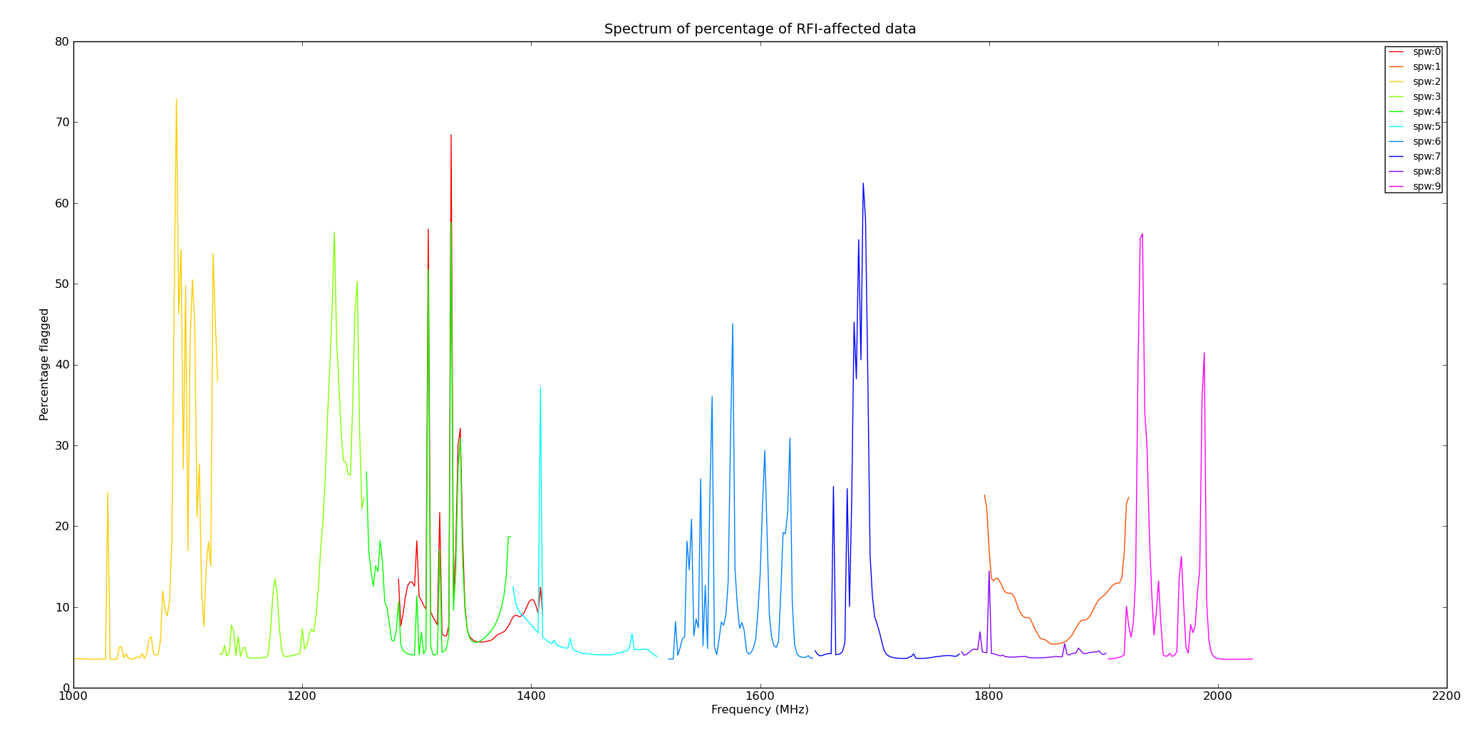Figure 14: Plots of the percentage flagged per channel : Dataset with 10sec timesteps.

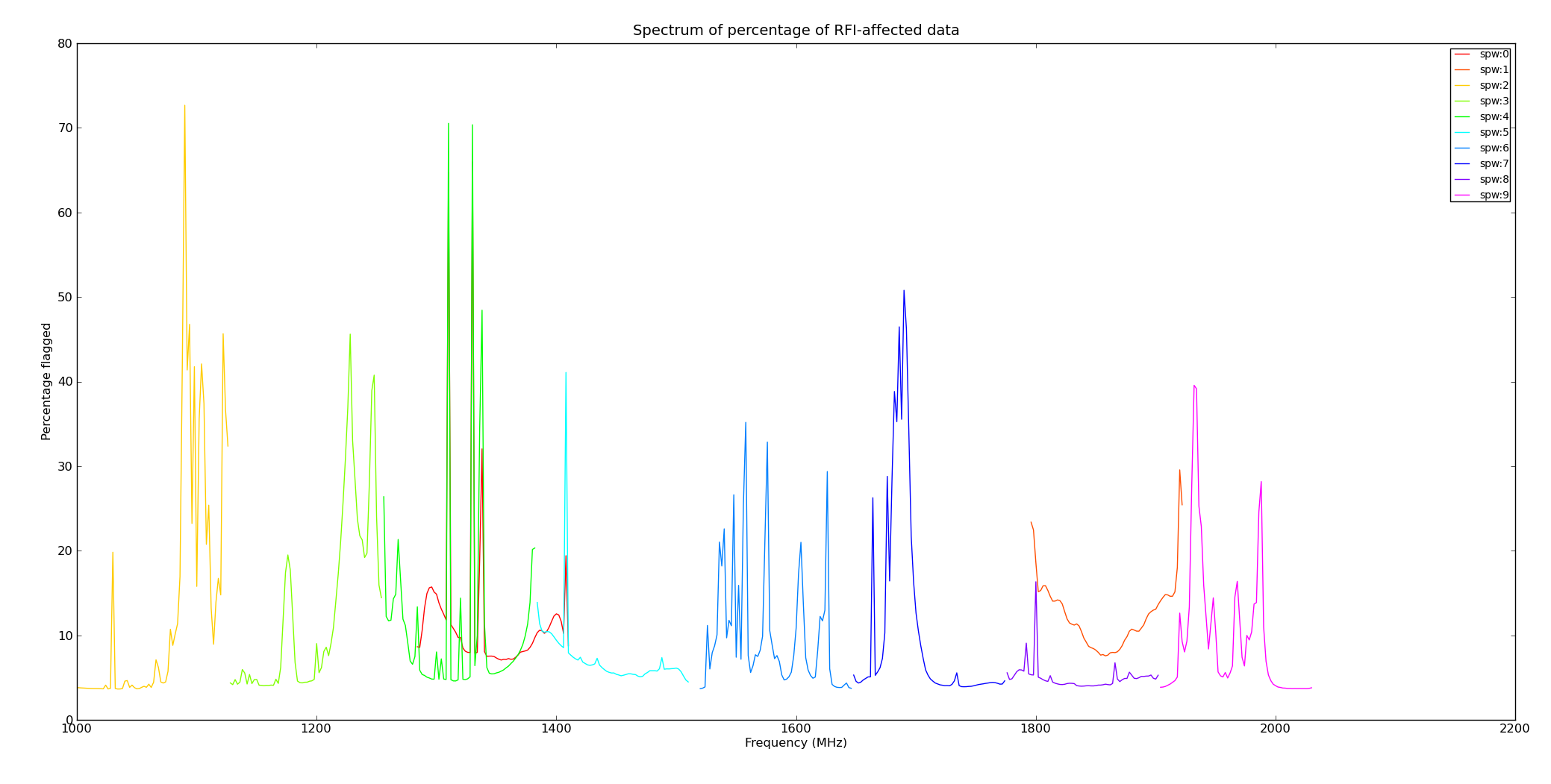Figure 15: Dataset with 1sec timesteps : Plots of the percentage flagged per antenna and scan. Each scan is about 1.5 minutes long. Flagging includes online flags followed by rflag running per scan. The left panel shows the percentage flagged per antenna, over all scans.

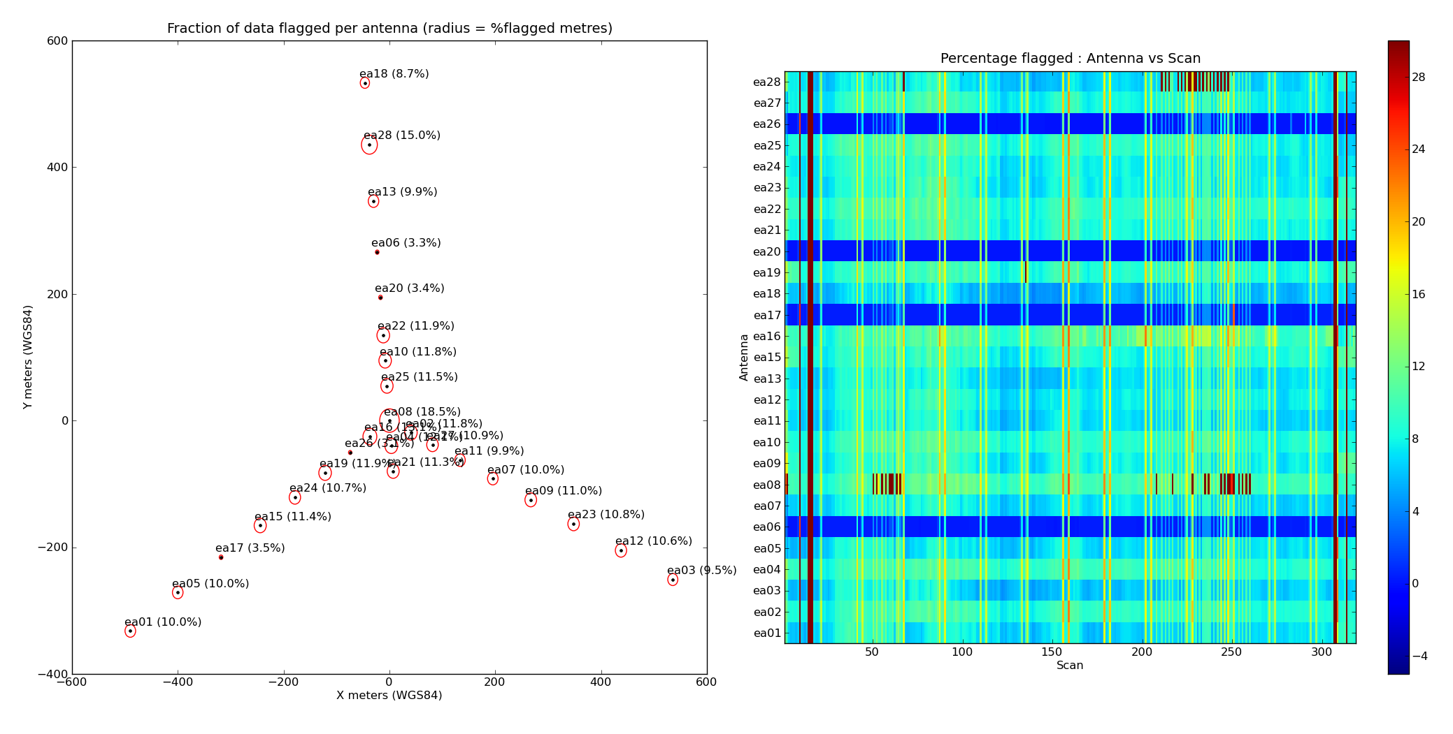Figure 16: Dataset with 10sec timesteps : Plots of the percentage flagged per antenna and scan. Each scan is about 1.5 minutes long. Flagging includes online flags followed by rflag running per scan. The data was completely unflagged before averaging to 10sec, to simulate averaging within the correlator.

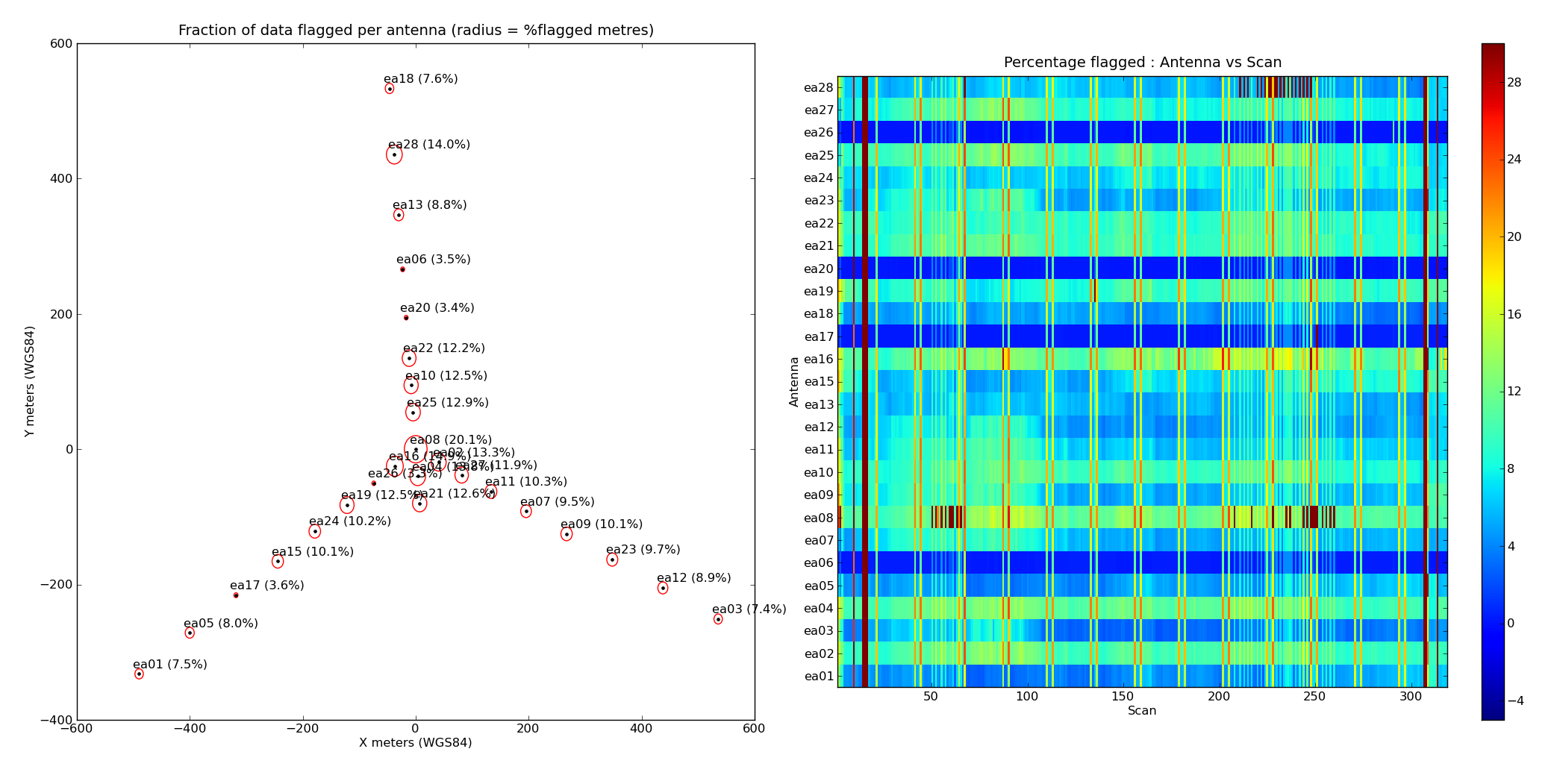Figure 17: Dataset with 10sec timesteps, with online flags applied before averaging from 1sec to 10sec. Plots of the percentage flagged per antenna and scan. Each scan is about 1.5 minutes long. Comparing with the previous two plots, again, there is very little gain (about 2% of data) of applying online flags before averaging to 10sec.

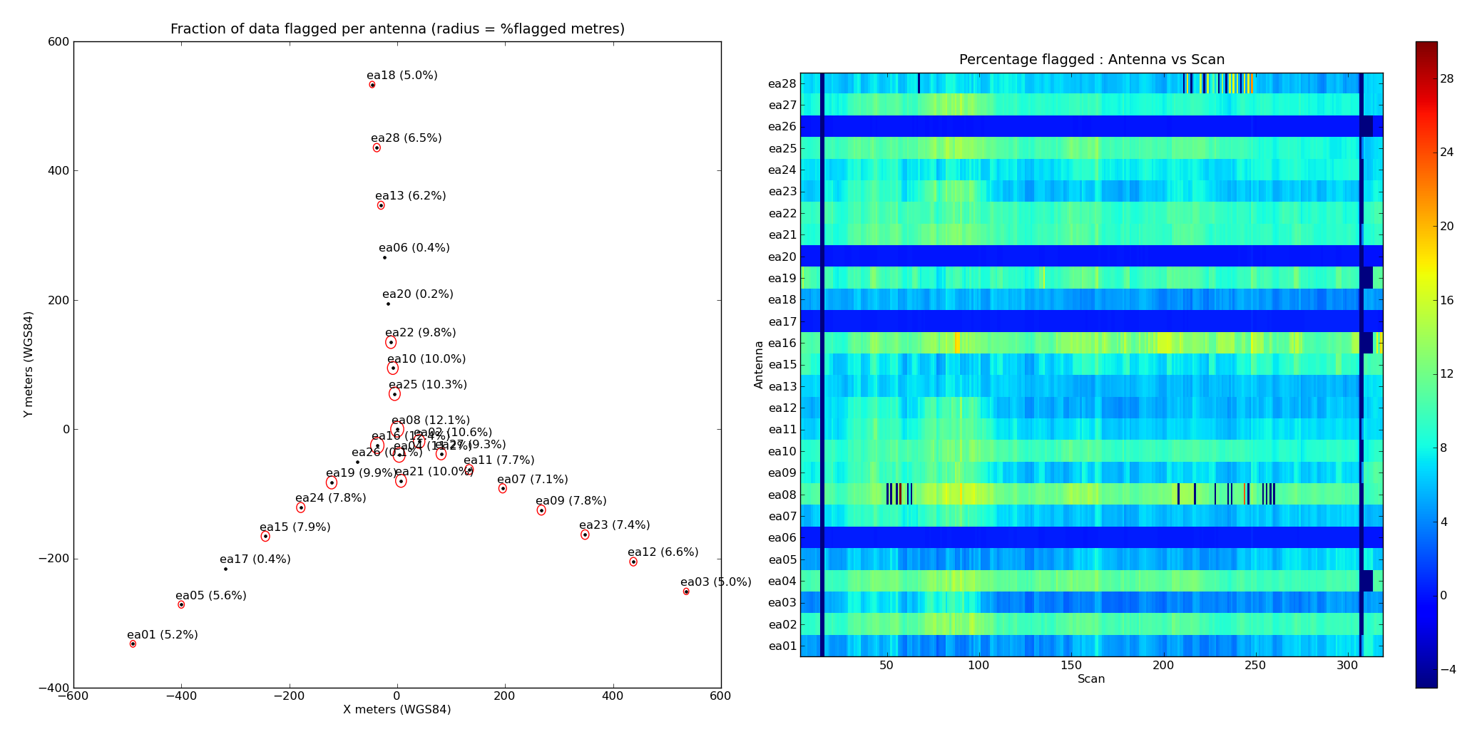Figure 18: Data amplitude vs frequency (flagged points are in red) for SPW=9, scan 7, and antenna EA11. (FIRST) : Result of rflag run on 1sec timestep data, and averaged to 10s only during plotting. (SECOND) : Result of rflag run on 10sec timestep data.