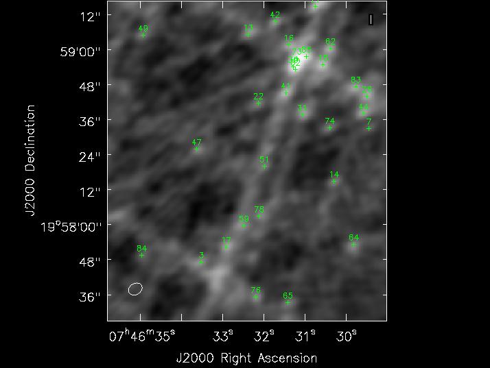
Figure 1: Image from Data with 100 point sources simulated in
Abstract
CLEAN [1] and dependent image plane deconvolution algorithms sometimes need restrictions to achieve convergence. Windowing, boxing, masking are some of the different names that have been used to describe the process of limiting the region of search for clean components and is usually a user based operation and some automatic algorithms are also in use with mixed results. The reason for needing masks is when a non masked image consists of more degrees of freedom that is available in the observations. All the operator(visually) based masking or automatic algorithm are high intensity locations mechanism and windowing around those avoiding sidelobes. CLEAN by definition does part of that in its deconvolution process but then forgets the location of the previous high peaks while searching for the next peaks, hence the need of masking. In this note we show that giving CLEAN some kind of memory is enough for many cases and void the need of masking (either manual or automatic).
CLEAN and similar algorithms start diverging in some cases when searching and subtracting clean components over a given dirty image. The reason for this is understood intuitively but the how and when divergence will occur has never been proven rigourously (it is very difficult to do so as the number of independent measurements made with different baselines is hard to quantify generically).
The reason for divergences are due several reasons. A couple are the limited number of degrees of freedom available in the interferometric visibilities and also the accuracy of the PSF(Point Spread Function) used at each pixel . The unknowns we are solving for are the intensities at each pixel position. The longer track observations from the VLA for example do not need masking usually especially if we use a few Cotton-Schwab[2] (CS) major cycles to compensate for the inaccuracies of the PSF. But short track observations or fewer antennas or source with complex structures may sometimes be non convergent when deconvolving by either creating non existant sources or ending up with residuals being higher than the initial dirty images.
The process of masking effectively reduces the number of unknowns being solved for by blocking pixels from being solved for (basically assuming that these pixels are just noise dominated and no signal are going to be detected there). Masking is usually done by visually analysing the dirty image (or residual image) and locating the bright structures and draw regions around these and tell CLEAN to deconvolve these regions only. Unmasked in contrast has the whole image to look around for the next peak. After the bright sources are deconvolved, unmasked CLEAN will start looking for clean component all over the image and thus assign flux density in many pixels. The number of pixels to which flux is assigned may in some cases be larger of what can be constrained by the data observed thus the problems of CLEAN fake sources or artefacts.
The process of masking and deconvolution so far has been considered as seperate issues and with the advent of commonly using CS major cycles between minor cycles of cleaning has made masking needed only in some cases. CLEAN by itself also locates peak brightness just like an operator looking at a dirty image and drawing masks; then why do we need masking in any cases at all ? The answer is that masking limits the search for clean components around the original bright sources but unmasked CLEAN will search for components all over the image and forgetting where the bright sources used to be.
Hence the idea of a CLEAN with some memory.
Plain Högbom CLEAN and its variant like Multi-scale CLEAN[3] works as follows:
Now in CS style of deconvolution after n loops of the above which can be tolerated by the accuracy of the PSF used the clean components are used to predict model visibilities and subtracted from the original visibilities which is hen re-image to make a fresh residual image. This prevents errors of the PSF used at different positions to propagate.
Now rather than depending on the user or some automatic algorithm (which may sometimes not distinguish sidelobes effects from real source) to mask the image to apriori limit the region of the search at stage 1 above we can use the knowledge of the position of the previous peaks to bias the search for the next components. Step 1 above becomes locate peak in a weighted residual image. The weight image used is a function of the prior peaks found. And thus as we will show now in many (dare we say most ?) cases the need for masking is removed.
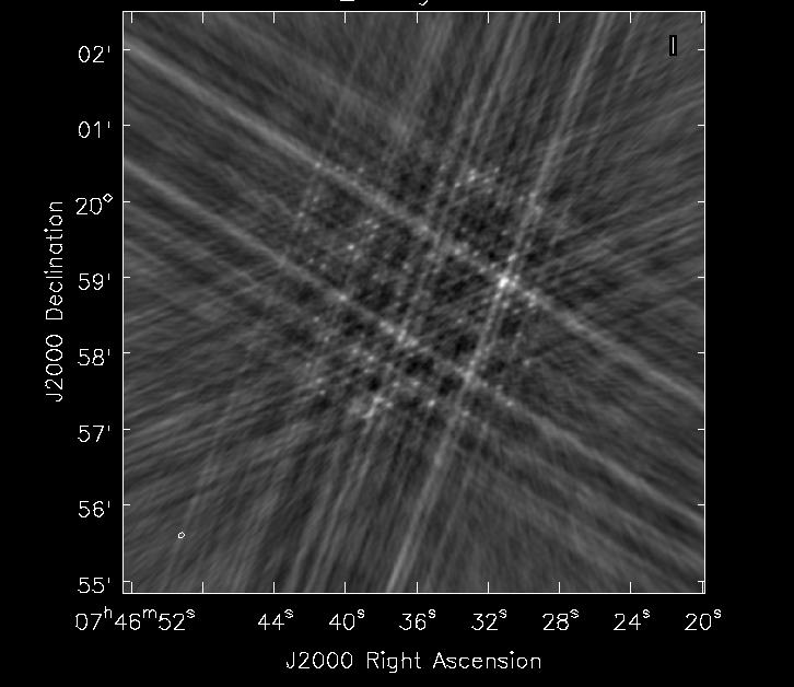
We used a real VLA B-array data set but we simulate 100 point random point sources in a blank field (See Figure 1).
Figure 2 shows a zoom in with position of sources labelled. As can be seen the confluence of sidelobes below source 3 and 17 may easily confuse auto masking or even human mask makers.
As we mentioned before for many cases we can live with such wrong masking as CS major cycles corrects for such initial wrong source estimates. But not always.
Now we perform a 5 major cycle CS style CLEAN; each major cycle is followed by a 300 component Högbom CLEAN with a gain of 0.3. See the results in Figure 3 and 4. In these figures the grey scale images are the restored images the green ’+’ markers mark the position of each simulated source and the red contours show where CLEAN searched for components.
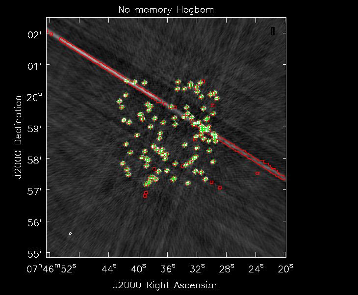
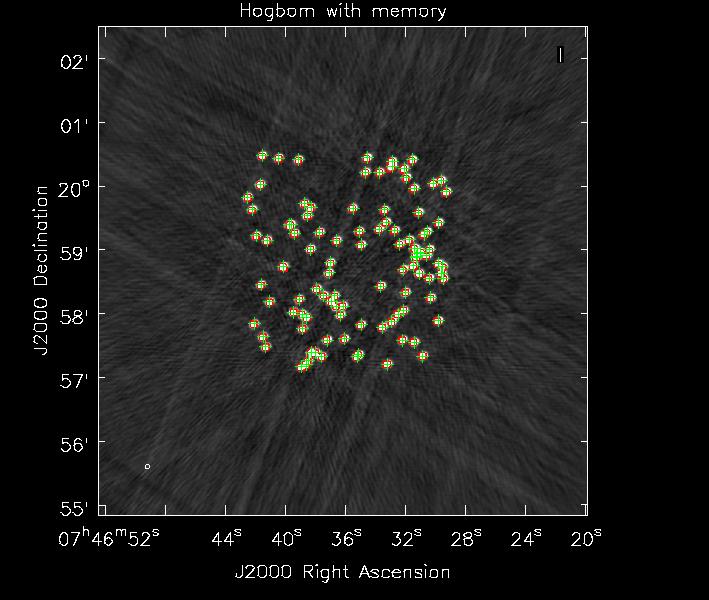
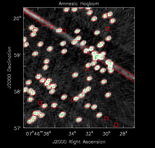
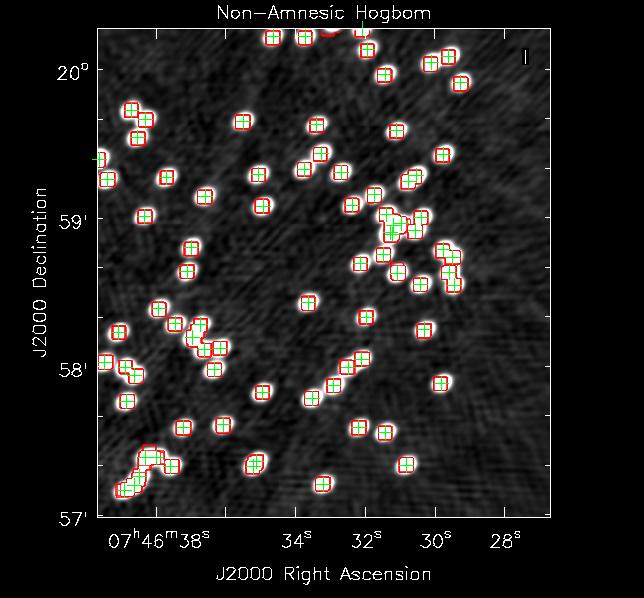
In this particularly agreessive minor cycle CLEAN stages we can see that the Non-Amnesic Högbom CLEAN concentrated its search for clean components where there are real sources only where as the normal Hgbom CLEAN has decided to look and put clean components along some sidelobe structures and some non-existant negative sources. To be fair if one were to just use a less agressive minor cycle (i.e more CS major cycles and lower gain in minor cycle CLEAN) the simple Hgbom clean converges to a final image with fidelity just like the Non-Amnesic algorithm. Just like with masking the Non-Amnesic algorithm allows one to be quite aggressive in most VLA imaging cases thus reducing computing time.
The idea is simple: while looking for peaks for the next clean component one should give preference to ones that are found close to a previously found bright source.
Let us consider a 2 dimension images, (x,y)is the location of a pixel
Now let us denote the residual image to r(x,y) and a memory image m(x,y). The memory image blank to start with (m(x,y) = 0).
The steps are as follows of how to locate the peak residual in a Non-Amnesic fashion:
Now as can be seen f(p) = 1 is just simple ordinary Högbom clean. We have initially implemented “weak”, “medium” and “strong” memory functions. We have seen that the medium memory works very well for most cases we have thrown at it. We believe the strong memory may be needed in cases where coverage is very poor like VLBI imaging for e.g. and low memory may be needed in low signal to noise fluffy structures.
In test code available in the deconvolver in CASA we have the following option
 f(p) = 1
 f(p) = 1 + 0.1 * p
 f(p) = p
 f(p) = p2
With the common usage of CS major cycles most imaging cases of telescopes like ALMA or the VLA do not need masking. But for many of the cases when masking is needed we have shown that deconvolution with a bit of memory of where the previous peaks were should be sufficient to void the need of interactive clean and such human time consuming processes.
[1] Högbom, J. A. 1974, A&A suppl., 15, 417
[2] Schwab, F. R; Relaxing the isoplanatism assumption in self-calibration; applications to low-frequency radio interferometry, AJ, vol. 89, 1984. 1076-1081 (The reference to Cotton-Schwab algorithm is to a paper “under preparation” on page 1078)
[3] Cornwell, T. J. 2008, Multiscale CLEAN Deconvolution of Radio Synthesis Images, Selected Topics in Signal Processing, IEEE Journal of (Oct 2008 Volume:2 , Issue: 5 , 793-801)