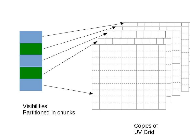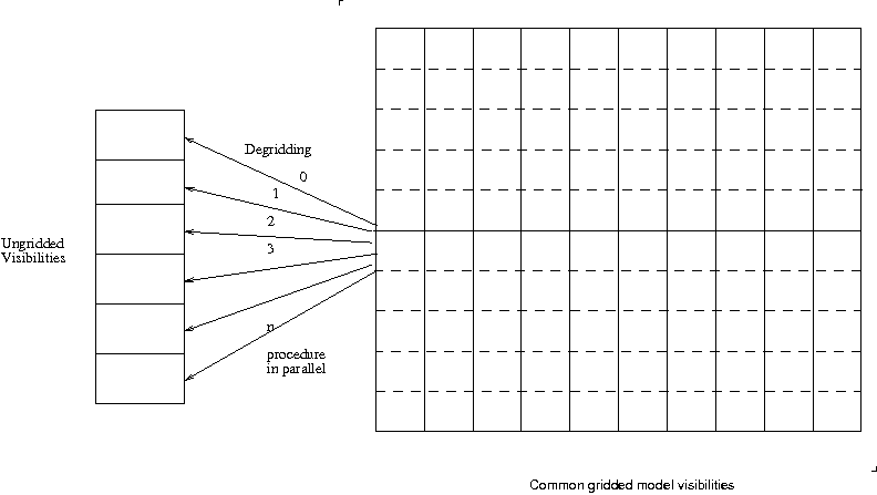
Figure 1: Data parallel degridding
Abstract
The most common interferometric imaging techniques in use involve gridding visbility data and Fast Fourier transforming (FFT). For large number of data sets especially those that are large and need convolutional correction the gridding stage is the largest time consumer (more than 75% in many cases).
We present some techniques of how to parallelize in shared memory mode the gridders and de-gridders without making copies of the grids or locking. We investigate issues that can prevent significant speed ups. We demonstrate by using some simple techniques that we can speed up degridding maximum 14 times (typical speedup time 13) and gridding with a miximum of 12 times (typical speedup time of 10) on a 16 core machine using multithreading. Some version of this algorithm has been implemented, using OpenMP multithreading, in production code of CASA[1] imaging since January 2012
Gridding: Simple interferometric imaging involves gridding visibility data onto a uniform grid and fast Fourier transforming. Even if we were not using FFT interforemetric imaging needs correction which uses projection algorithms (W-Projection[2], A-Projection[3] etc) which involve convolutions. In typical high quality interferometric imaging degridding is performed to do a Cotton-Schwab style major cycle. Degridding is the process of predicting from a model image what would be the visibilities measured at the different uv-points sampled by the interferometer.
The larger the convolution functions used the more compute intensive and time consuming the gridding and degridding sections are.
In this model different pieces of the uv data is sent to be gridded and degridded seperately. For degridding it is the obvious way to parallelize and there is not much extra overhead as compared to single thread or process degridding. The visibility data to be predicted can be partioned in n equal parts and distributed to the threads (or processes) and the same grid which contains the gridded model visibilities is shared by the n processes. No locking is needed as the common grid is “read only” and the prediction happen on independent data pieces. For load balancing the partition of the ungridded visbilities need to be equal in processing time. If the distribution of size of convolution function used to degrid the data is quite random and distributed evenly across each data partition then just uniform partitioning will be load balanced and near linear speedups can be expected. For mosaicing or wprojection (with the VLA) for example this is the case for partitioning over a few integrations in time.
We can grid in a “data parallel” way too and it is the obvious choice for cube imaging as the cube can be partition on channel basis and the data is partitioned along the spectral axis so that only the section needed by each sub-image is read by a given thread/process and gridded independently.
For continuum image the direct data parallel processing involves copies of the grid which is then combined in a weighted average after the children have processed it all.
For large images this means that memory for n complex grids need to be available for n threads/processes to proceed (n×Npixels × 16 bytes) . On multiple nodes this is very doable but many node now comes with 16 or 32 physical CPU’s thus having 32 double precision complex grid in RAM may not be an option on a single node.
Pseudo code for a grid copies multi process gridding would look like the following:
The other option is to have one grid but each child process grid the data partition with locking of the grid. This will be mostly serial. This is where a non-data parallel but common grid method may work as we show in the following sections
Instead of partioning the data for gridding; for each iteration of “data read”, share all the data among the threads/processes. This step does not cost anything extra on shared memory parallelism (e.g multithreading). The output grid is commonly shared too but each process/thread is assigned exclusivity on a section of the grid. The child then proceed to grid only the data from the common data that falls on its assigned section
As a reminder, single process gridding proceeds as follows:
Now instead the grid is shared among all the threads/processes but each is assigned exclusive regions of the grid to perform gridding onto. All the visibility data is commonly shared among all threads. Then multi threaded gridding will proceed as follows:
As can be seen by pseudo code above there is no copy of grid and no locking involved. The extra work introduced is to check if a piece of data contribute to a section of a grid or not. If that check is much smaller in cpu cycles than the convolution part then it does not contribute much to the whole scheme.
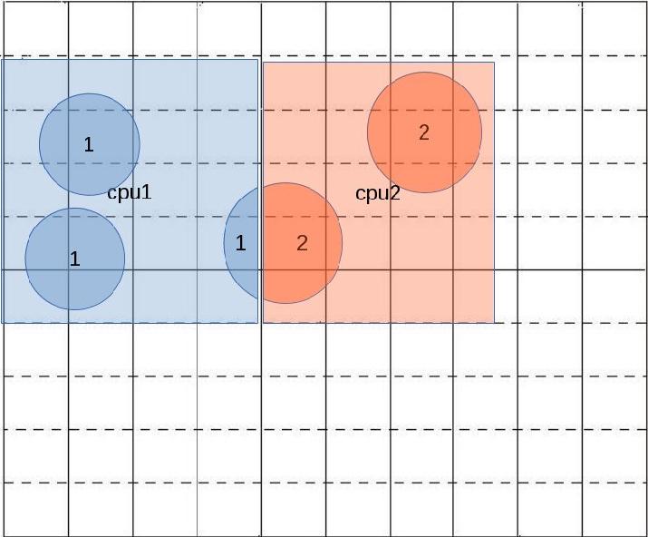
As can be seen from Figure 3 each cpu is assigned exclusive write access to adjoining sections with no evrlap.
The algorithm for gridding is: each cpu goes through all the visibility data and grid the data that fall in their respective grid. When the data point with convolution function covers 2 or more sections then the cpu add to the grid only the part that falls within its borders.
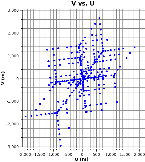
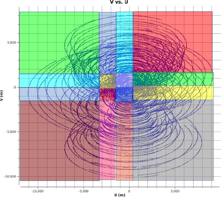
Each chunk of data that are read into memory may have different uv distribution pattern largely dependent on how the data is stored and loaded in chunk. Telescopes like VLA and ALMA tend to store the data at every integration. Thus a given integration snapshot of uv distribution tend to span quite some area over the working grid (see Figure 4)
So for the VLA or ALMA the algorithm to give exclusivity to each CPU can be based on uv based sectioning of a one or a few integrations of visibility data.
Like any parallelization solutions load balancing is important or else the gain hoped is not seen.
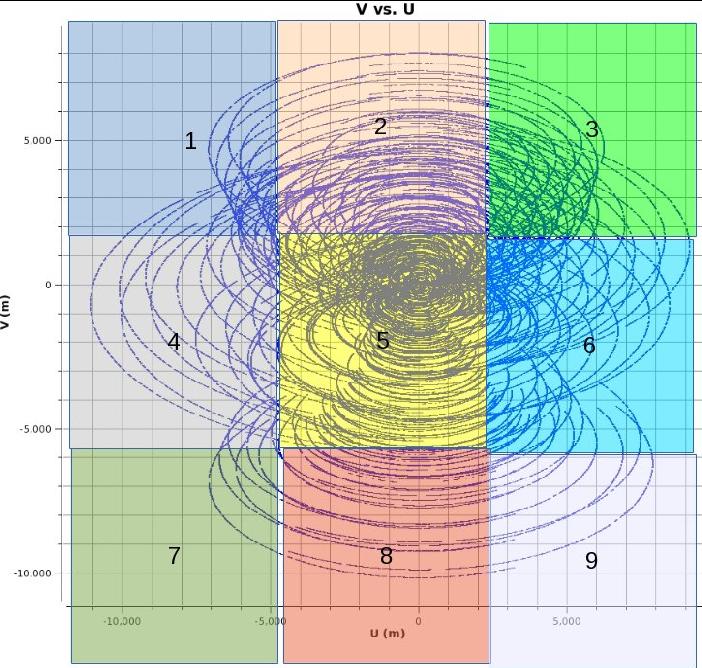
In figure 5 we show a simple uv area based partitioning dependent on the grid size only (the line tracks are uv tracks of baselines over some integrations in time). As can be seen the number of uv points in each partition varies a lot. The CPU that gets Partition 5 will have the most crunching to do while the CPU that gets partition 7 does not have much to do. If for example this is a 2 CPUs system then it will load balance itself as one cpu is crunching on partition 5 the other one can go through the others...but if it is a 9 CPUs system then most of the CPUs would be idling except for the on working on 5 and the speed up will be not much from serial. So having more partitions than CPUs may naturally balance the work load. The issue then is if the ratio of “checking if it is my partition” to “de/gridding work” becomes significant in CPU cycles used then speedup is lost. So just blindly making many small sectors and distributing it among CPUs may not always be the solution
So depending on the situation a more adaptive scheme for partitioning is needed.
For example for a 8 or 16 CPUs system a density dependent partitioning like in Figure 6 can be
adopted to achieve some good speedup from serial.
In fact density distribution over time for telescopes like the VLA and ALMA varies slowly as tracking over the sky is done. The sum of weights while gridding is a marker of how much is being done while gridding (and degridding). Thus once in a while during the gridding process the sum of weights for different partitions can be monitored and if the sum of weights become wildly different an adjustment in partitioning can be done.
One scheme that works very well is try different partition for a few integration and pick the one that goes fastest and usually that works fine for a couple of hours of data and recheck again later.
Other schemes can be devised for example known arrays the UV tracks at given AZ-EL observation are predictable thus we can have predetermined partitioning done for N cpus used.
This is for parallelization with openmp specifically. Although dynamic scheduling has larger overhead it works better in the case of gridding and degridding specially if many small partition are used. Static scheduling has very little overhead and in some implementation a loop number is assigned to a thread quite early and locked. This may mean that a given cpu may get a few grid partitions that has not much to do whereas another one may get too many dense partitions. Experimentations on VLA data mostly has shown dynamic scheduling to achieve better or equal speedups in all cases tried.
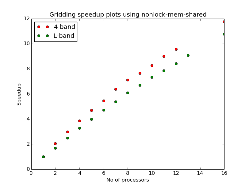
In applying some of the techniques above we can get speedups of upto 12 in gridding
on a 16 core machine gridding B-array VLA data. Speedup being defined here as  where T1is the time taken for a single process and TNis the time taken by
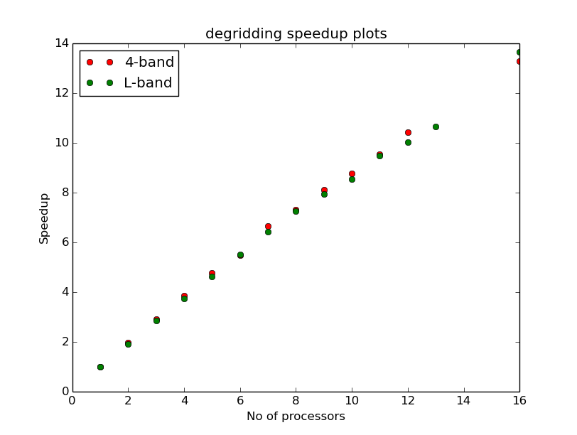
N-processes or threads. The plots in Figure 7 and Figure 8 are for w-projection
gridding and degridding on 1.4GHz and 74 MHz datasets.
where T1is the time taken for a single process and TNis the time taken by
N-processes or threads. The plots in Figure 7 and Figure 8 are for w-projection
gridding and degridding on 1.4GHz and 74 MHz datasets.
[2] Cornwell,T.J.;Golap, K.;Bhatnagar, S., "The Noncoplanar Baselines Effect in Radio Interferometry: The W-Projection Algorithm", Selected Topics in Signal Processing, IEEE Journal of (Volume:2 , Issue: 5 ) , 2008, pp.647 -657
[3] Bhatnagar, S.; Cornwell, T. J.; Golap, K.; Uson, J. M., “Correcting direction-dependent gains in the deconvolution of radio interferometric images”, Astronomy and Astrophysics, Volume 487, Issue 1, 2008, pp.419-429