Guide to Spectral Line/Astrometry VLBA Tutorial
Please note before you start:
- This tutorial is specifically for the 15th Synthesis Imaging Workshop. You must use the account which is assigned to your computer or AIPS will not work. The data is in ~/vlba:
- BM272HC.fits (12 GB): Date containing target and calibrators.
- BM272HC_geodetic.fits (0.3 GB): Data containing geodetic block. These are observations of many calibrators around the sky. There are 3 ~half hour blocks of calibrators observed ant the begining middle and end of the observation.
The geodetic blocks are in a different file from the target because they have very different frequency setups. The geodetic block require to have widely spaced frequencies with a single polarization in order to measure the multi-band delay (MBD). The target dataset is dual polarization (important since the source is circularly polarized) and frequencies that are continuous.
MAKE SURE YOU ARE RUNNING THE CORRECT TASK ON
THE CORRECT DATASET!
- Details on what you are doing and why can be found in AIPS Memo 110: Strategy for Removing Tropospheric and Clock Errors using DELZN.
In short, to obtain precise positions and
good image quality with phase referencing in VLBI, two things are needed; a close
calibrator to the target source to minimize atmospheric differences between the target and calibrator and a good correlator model.
The VLBA correlator uses a model for the troposphere
computed from seasonal models as well as the best estimates
of the clocks, positions of each antenna and earth orientation parameters.
This major source of error produces a systematic phase
difference between the calibrator and target which limits the target
positional accuracy and image quality. The troposphere model error,
however, can be estimated by observing about ten calibrators over the
sky over a 30-minute period, and then calculated the erroneous delay. So with
this tutorial you will:
- Calibrate the regular data all the way through imaging (see Appendix C. in the AIPS Cookbook).
- Calibrate the geodetic style data through instrumental delay removal.
- Compute the Multi-band Delay (MBD). The MBD is a function of a variable clock delay, and a troposphere
term (zenith path delay) which has a well-defined function of elevation (called a mapping
function), times an unknown constant.
- Use the AIPS task DELZN to fit the MBD and calculate the clock and
zenith path delay error.
- Apply these corrections to the dataset that includes the target.
- Image the target and see an improvement over not doing the geodetic calibration.
- Also I am only giving the important inputs to task. The other inputs should
be default. An easy way to set all the inputs to the default in a task is
to type "default taskname".
- A more thorough description of how to reduce VLBA data can be found in the AIPS Cookbook Appendix C.
- This is an observation of water masers in star-forming region IRAS 00420+5530 and involves phase referencing. The sources in the observation are as follows:
- AFGL2591 - phase calibrator/target (mazer source for which the position is desired)
- J2007+4029, 20330+40003, 20327+40396, 20324+40574 - calibrators that are phase referenced to AFGL2591 (note that only J2007+4029 and 20330+40003 are detected).
- 3C345A, 3C454.3A - fringe finders, bandpass calibrators
- numerous geodetic calibrators that I will not name.
- This data was published by Rygl et. al.
- For a comprehensive overview of AIPS see the AIPS COOKBOOK, especially Chapter 3:Basic AIPS Utilities and Chapter 12:AIPS for the More Sophisticated User for the basics. Chapter 9:Reducing VLBI Data in AIPS is the chapter explaining VLBI data reduction, but it is rather overwhelming so Appendix C:A Step-by-Step Recipe for VLBA Data Calibration in AIPS is recommended as a first step. However, below I summarize some useful commands (in parenthesis are the short form of the command):
- getname (getn) catalog #: get the name of catalog # and put in INNAME, INCLASS and INSEQ. Other similar: geton (get outname); get2n (get in2name); get3n (get in3name) etc..
- input (inp) taskname: show the inputs of taskname.
- tget taskname: get a task and fill in the inputs of the last time the task was run.
- ucat (uc): list uvdata catalog.
- mcat (mc): list map catalog.
- tvlod (tvlo): load an map onto the TV.
- tvinit (tvin): initialize and clear TV.
- imhead (imh): Print the file header (this can be used on both uv data and images despite the name). This will list informative things like the date of observation and the number and types of tables attached to the data.
Instructions for general spectral line/phase referencing data reduction
Start AIPS with the command aips tv=local and using AIPS number 15
- Load the data with FITLD. The spectral line data has been preloaded because it takes a while to load. If you type "uc" you will see a file named "BM272HC.FPOL2.1". So you only need to load the geodetic data.
default 'fitld'
clint 0.25➜ set CL table interval to 15 seconds.
datain '/var/nrao/vlba/BM272HC_geodetic.fits➜ this is not a typo, you must leave off the close ' or AIPS will capitalize the everything within the ' ' and you will get an error because FITLD will not be able to find the directory.
outname 'BM272HC GEO'
inp
go
- Look at the structure of the data with LISTR. This will give you a listing of the scans as well as the source and frequency structure in the observation.
default 'listr'
getn BM272HC FPOL2 file
optype 'scan'
docrt 1
inp
go
- Load in the VLBA data reduction procedures: see EXPLAIN VLBAUTIL for full
description of procedures. Procedures are run by just typing their name, rather than using "go".
run vlbautil
- If you get a BLEW CORE or other similar error message, you have filled your procedure memory (VLBAUTIL is very large and loading it three times will do this). To fix it type restore 0 then reload VLBAUTIL
- Fix ionosphere contribution to the dispersive delay by running VLBATECR.
default vlbatecr
getn BM272HC FPOL2 file
inp
vlbatecr ➜ to run VLBATECR
- Fix earth orientation parameters by running VLBAEOPS.
default vlbaeops
getn BM272HC FPOL2 file
inp
vlbaeops
- Correct sampler threshold errors from correlator by running VLBACCOR.
default vlbaccor
getn BM272HC FPOL2 file
inp
vlbaccor
- Now lets take a look at the fringe finders by running VLBACRPL. VLBACRPL runs POSSM and displays the spectrum of each baseline (to Fort Davis (antenna 2)), with the amplitude on the bottom and the phases on the top.
default vlbacrpl
getn BM272HC FPOL2 file
stokes 'half'
refant 2
gainuse 4
solint -1
dotv 1
source '3C345A' '3C454.3A'
inp
vlbacrpl
As you can see the 3C345A has very strong fringes.
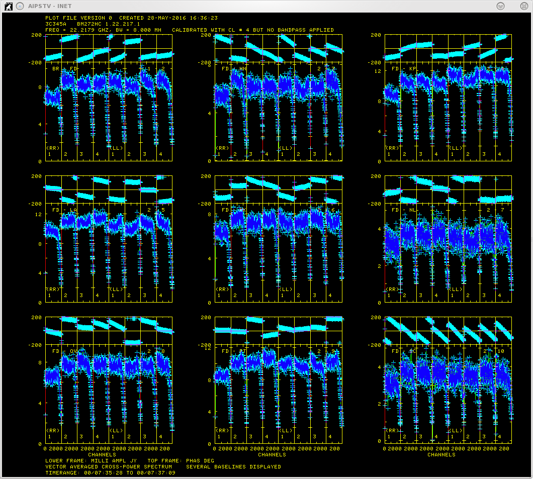 So we will use it was the calibrator to set the instrumental delays.
- Find and remove instrumental delay by running VLBAMPCL.
default vlbampcl
getn BM272HC FPOL2 file
calsour '3C345A''➜ strongest source.
timer 0 07 35 28 0 07 37 09 ➜ scan with good fringes we found in POSSM plots.
refant 2➜ choose reference antenna from in the middle of array, FD (antenna 2) is a good choice.
gainu 4➜ apply highest CL table. Please do an imh here to make sure the highest CL table is really 4.
inp
vlbampcl
At this point you should check on the calibration:
- First check you have no failed solutions. At the end of the FRING run it should tell you how many "good" and "failed" solutions it has found. For this step there must be no failed solutions, failed solutions in this step mean that whatever antenna the failed solution was on is deleted from your data. For this data there should be "80 good solutions".
- check solutions in POSSM, the jumps in phase between the IFs should be gone. The phases may also be flattened.
tget possm➜ to "get" all the inputs from the last run (it was run when we ran the procedure VLBACRPL).
gainu 5
inp
go
As you can see the the phases for 3C345A have been flattened and the phase jumps between the IFs are gone.
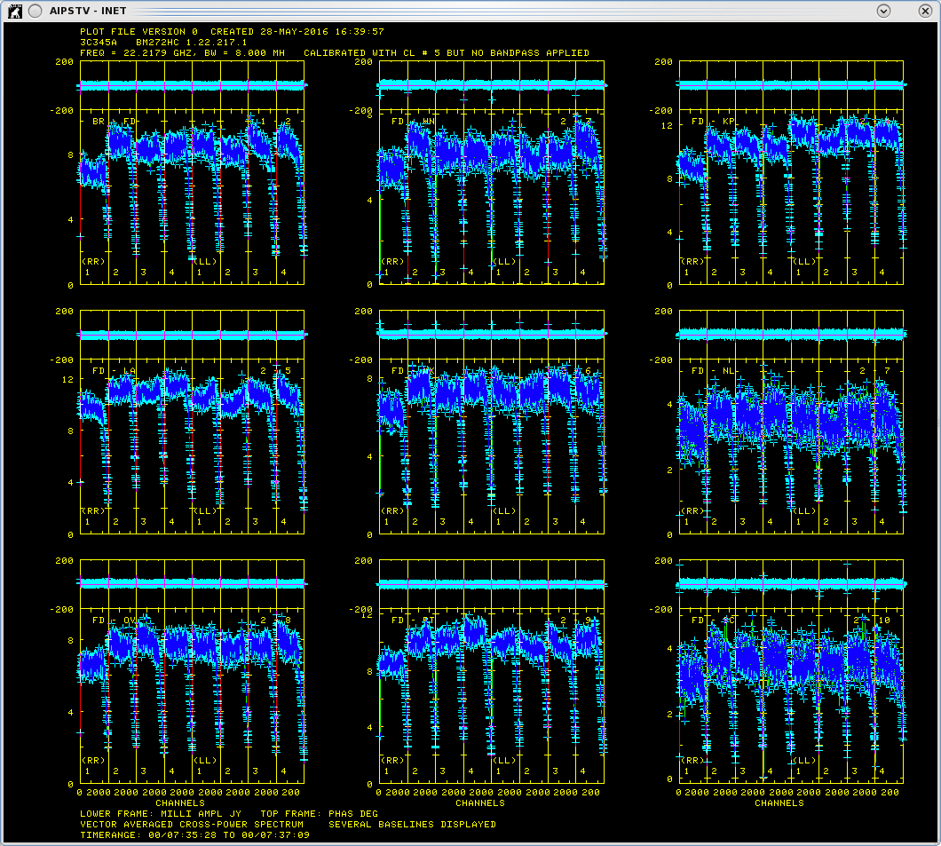 For other sources farther away in time the phases may be different from 0 but there will still be no phase jumps.
- Calibrate bandpass shape with VLBABPSS.
default vlbabpss
getn BM272HC FPOL2 file
calsour '3C345A' '3C454.3A'➜ use both very strong sources as bandpass calibrators.
refant 2
inp
vlbabpss
Now check the bandpass solutions with POSSM (tget possm; baseline=0; aparm(8)=2; aparm(9) 1; bpver=1;doband=1). The solutions should look like a reasonable fit of the bandpass shape. 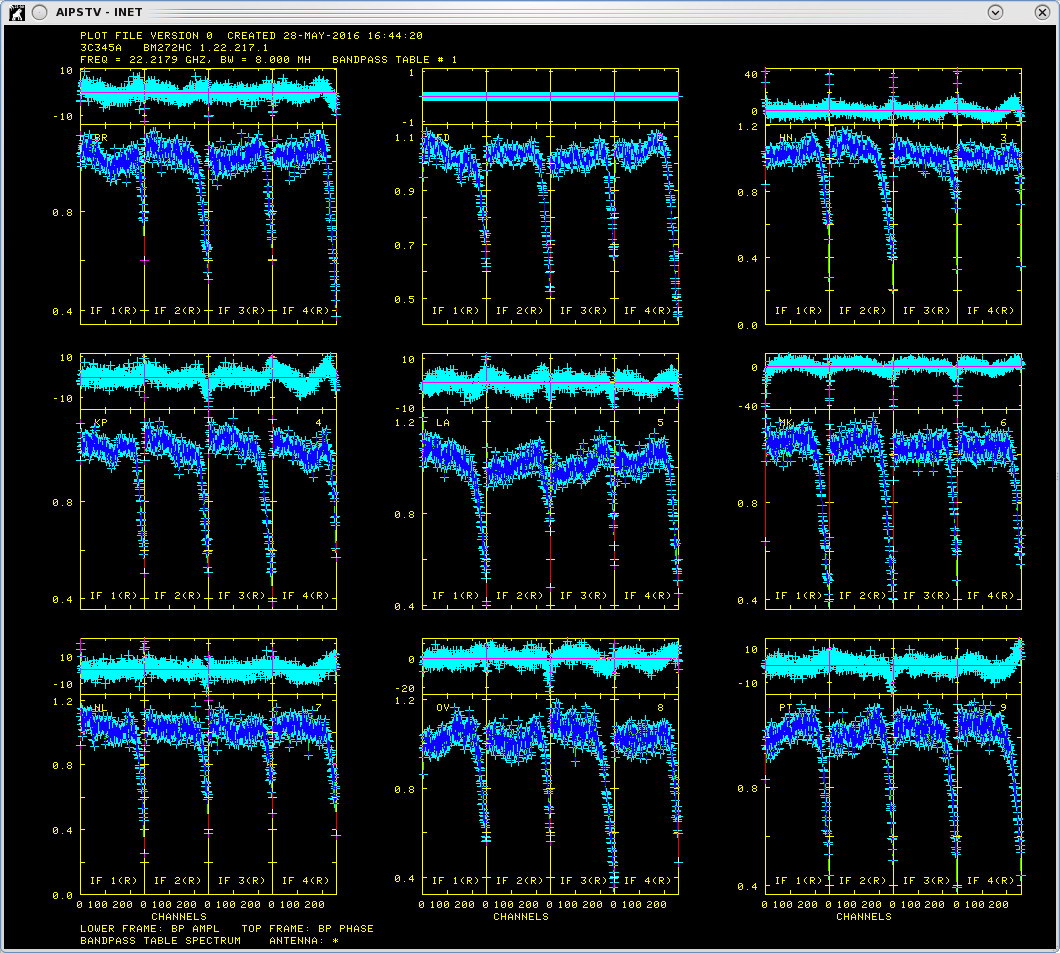
- Perform amplitude calibration by running VLBAAMP.
default vlbaamp
getn BM272HC FPOL2 file
inp
vlbaamp
- Examine amplitude calibration by running SNPLT.
default snplt
getn BM272HC FPOL2 file
dotv 1
inext 'cl'
invers 7
opty 'amp'
nplots 10
opco 'alsi'
do3col 1
inp
go
The amplitude gains change with over time as the sources rise and set, with higher gains at lower elevations, also because 3C345 and 3C454.3 are so strong, they also increase the gains. 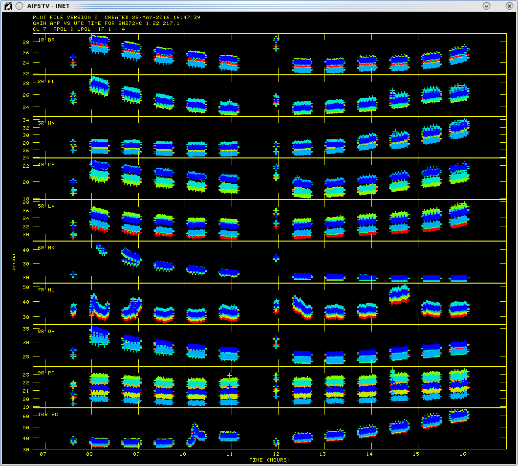 The different IFs and polarizations (RR and LL in this case) are shown as different colors.
- Fix parallactic angle by running VLBAPANG.
default vlbapang
getn BM272HC FPOL2 file
inp
vlbapang
- Edit the data using EDITR on each source separately.
default editr
getn BM272HC FPOL2 file
docal 1; gainuse 0 ➜ calibrate data with highest CL table.
crowded 1 ➜ to plot all polarization and IFs on top of each other.
do3col 1
doband 1
bpver 1
flagver 1
outfgver 1
antuse 1 2 3 4 5 6 7 8 9 10 ➜ to plot all the baselines to one antenna at the same time.
Run on one source at a time:
source 'AFGL2591''
inp
go
source '20330+40003''
go
source 'J2007+4029''
go
Note that the data looks great and there are a few high points to flag. EDITR plots both amplitudes and phases, so this is a good way to just look at your data. If you plot the phases on all the baselines, note that you can see coherent phases on J2007+4029, but not the other two sources. AFGL2591 has strong mazers that fringe, but EDITR is plotting all the channels averaged. Flag high points using "Flag time". Here is an example of a high point 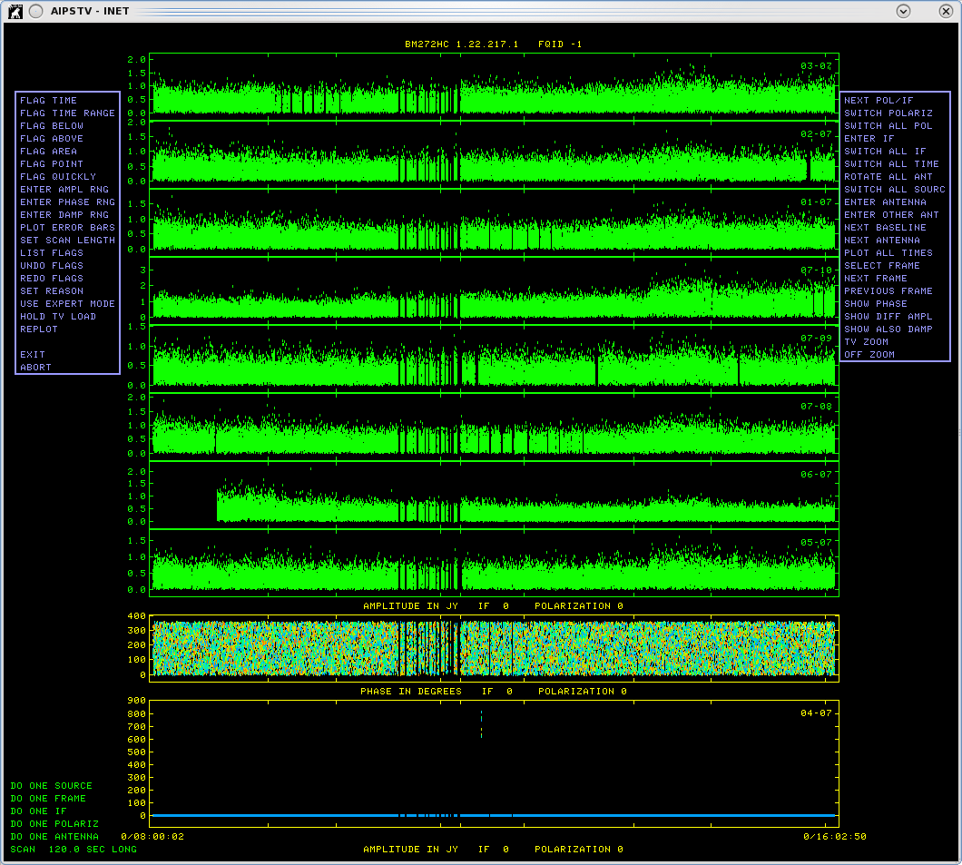 , it flagged
  and after rescaling with "Replot" to make sure there are no more bad points
 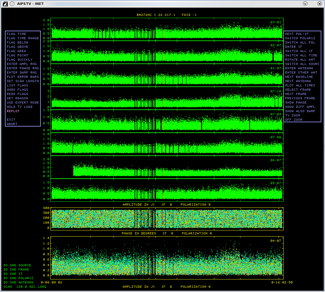 .
.
- Save calibration up to this point with TASAV. TASAV makes a new file with all your calibration tables, this is very useful because it contains everything you need to recalibrate your data in a very compact form. It is also a good idea to do this before you do anything you are unsure about or will change important tables (AN, SU) in ways that are hard to change them back. In the next step we are changing the SU table.
default tasav
getn BM272HC FPOL2 file
inp
go
- Shift the position of AFGL2591 with CLCOR. The observed/correlated position of AFGL2591 was quite wrong and shifting a large distance in the image plane is quite imprecise, therefore it is important to shift the uv-data with either CLCOR or UVFIX. Normally you would reduce and image the data to find the shift.
default clcor
getn BM272HC FPOL2 file
sour 'AFGL2591''
gainver 8
gainuse 9
opcode 'antp'
clcorprm(5)= 0.009
clcorprm(6)=-0.129
inp
go
Note: If you do something wrong in this step, just doing the same shift in reverse will not undo the shift to astrometric accuracy due to the complications of precession. This is why we did the TASAV step. To undo the shift, delete the CL table that was created by CLCOR and the SU table using extd. Then copy the SU table from the TASAVed file with TACOP.
- Apply all calibration up to this point and copy out IF#3 with SPLAT. The mazers are in the 3rd IF and we will be fringe fitting on that mazer so we should get rid of the other IFs. We could have gotten rid of the other 3 IFs earlier, but I kept them around for two reasons, 1) I wanted you to see what more than one IF looked like in displays and editing since most of the data you will receive will be more than on IF; and 2) it is a good idea to apply the calibration after the position shift and before global fringe fitting (and adding the zenith delay correction).
default splat
getn BM272HC FPOL2 file
bif 3; eif 3
docal 1
gainu 9
doband 1
bpver 1
inp
go
For the next 4 steps (17-20) you will be running the AIPS tasks on the dataset out of SPLAT. It should be BM272HC.SPLAT.1.
- Select channel for global fringe fit with POSSM.
tget possm
getn BM272HC SPLAT file
sour 'AFGL2591''
base 2 0
gainu 0
solint -1
doband -1
aparm 0, 1, 0, 0, -180, 180, 0, 0, 1
dotv 1
nplots 1
bchan 100; echan 180
inp
go
We really only need to look at one spectrum for this, so you can hit "D" right away or go through a few to see how the spectrum changes a bit from baseline to baseline. 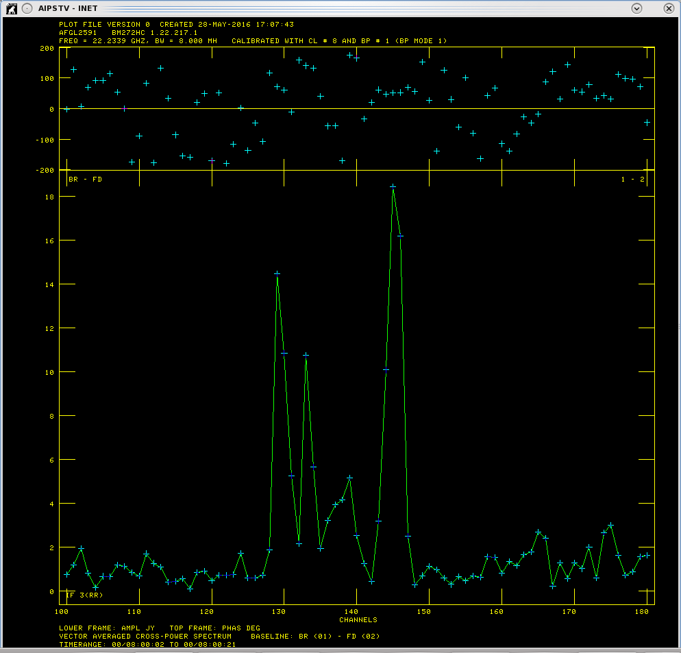 shows that the mazer is strongest in channel 145.
- Perform a global fringe fit with FRING. The following steps through imaging are not strictly necessary since we will have to redo them once the geodetic calibration is done, but is an excellent way to check the calibration up to this point is correct.
default fring
getn BM272HC SPLAT file
calsour 'AFGL2591''➜ do a global fringe fit on mazer.
bchan 145;echan 145
refant 2
search 2 9 5 4 1 3 7 8➜ list of antennas to search if a solution is hard to find.
aparm(9) 1➜ do exhaustive baseline search.
docal 1; gainu 0
inp
go
I got "Found 4498 good solutions" and "Failed on 42 solutions", you should get something similar but not necessarily exactly the same number of good and failed solutions. Some failed solutions are fine at this point.
Hint: We will have to do this exact same step after doing the zenith delay calibration so it is helpful to save the inputs to FRING. This can be done with vnum and vput.
vnum 1; vput fring
- Interpolate the fringe solutions with CLCAL.
default clcal
getn BM272HC SPLAT file
gainv 1➜ CL table with all the calibration.
gainu 2➜ CL table to write next step of calibration in.
snver 1➜ smoothed table out of SNSMO, contains final fringe fit.
interpol '2PT'➜ use 2PT interpolation.
refant 2
sour 'AFGL2591' '20330+40003' 'J2007+4029'➜ sources to which to apply calibration.
calsour 'AFGL2591''➜ phase calibrator, phases will be applied from AFGL2591 to itself, 20330+40003 and J2007+4029.
inp
go
This is another spot where vnum/vput will be useful:
vnum 1; vput clcal
- Apply calibration and make single source data sets with SPLIT. I like to work with single source files, it's less confusing, especially when self-caling and imaging.
default split
getn BM272HC SPLAT file
freqid 0
docal 1; gainu 2➜ apply calibration; from CL#2.
sour 'AFGL2591' '20330+40003' 'J2007+4029'➜ split out target and phase calibrator.
inp
go
This will produce three files named isourcename.SPLIT.1.
- Image AFGL2591 with IMAGR.
default imagr
getn AFGL2591 SPLIT file
bchan 125; echan 150; nchav 1; ➜ image channels 127-150.
cell 3e-5; imsi 1024➜ cell size of 0.03 mas; image size of 1024x1024.
dotv 1; niter 1000➜ do interactive clean; with 1000 iterations.
inp
go
You can try autoboxing this works reasonably well:
im2parm 10 6 9 0.5➜ only do 10 boxes per major cycle; find islands with > 6*rms; box is accepted if peak > 9*rms; box is accepted if its peak brightness is >0.5*max residual.
go
HINT:First few channels will not have any masers, just hit "STOP CLEANING"
until you see some emission.
Look at cube with TVMOVIE and use SQASH (bdrop 3; dparm 1 0) to collapse cube
and then use TVLOD to look at the SQASH image 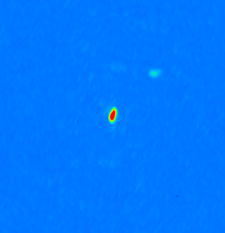 .
.
- Image J2007+4029 and/or 20330+40003 with IMAGR to make sure phase referencing worked.
default imagr
getn J2007+4029 or 20330+40003 SPLIT file
bchan 0; echan 0; nchav 256; ➜ average all channels.
cell 1.5e-4;imsi 2048➜ larger image size because sources might not be at center of field.
dotv 1; niter 1000➜ do interactive clean; with 1000 iterations.
inp
go
Image of J2007+4029 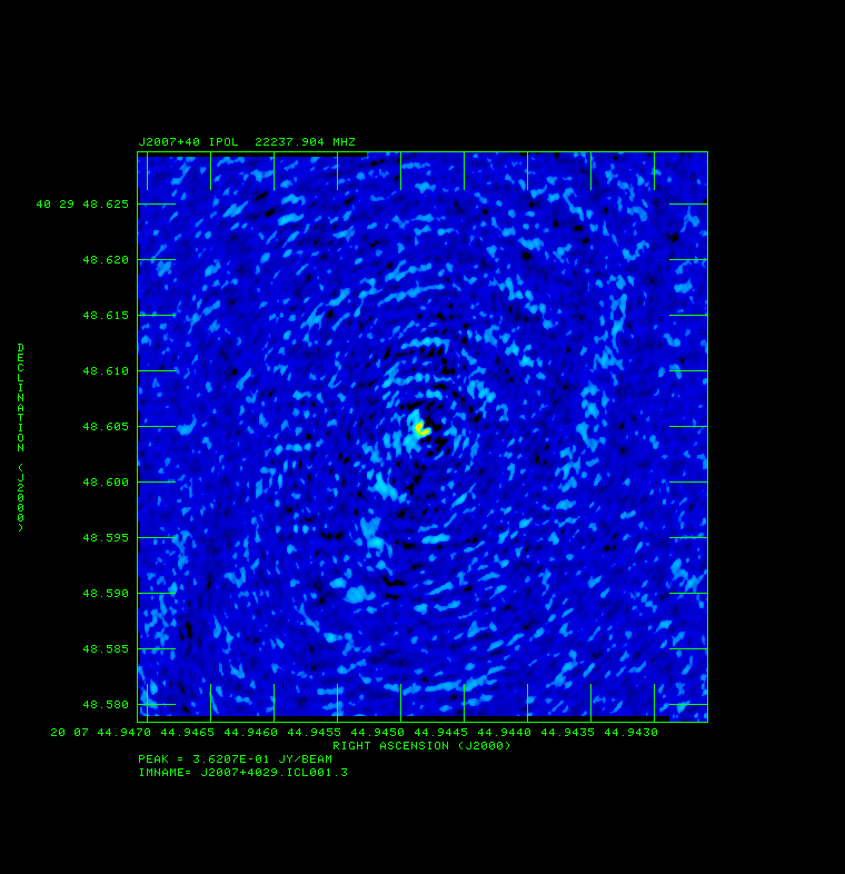 .
.
Instructions geodetic-like calibration to improve astrometry (and phase referencing).
We start with the same steps 4-8 as above on the
geodetic data. It's name should be something like "BM272HC GEO.UVDATA.1" if you followed the naming I suggested in the FITLD step above.
- Fix ionosphere contribution to the dispersive delay by running VLBATECR.
default vlbatecr
getn BM272HC GEO UVDATA file
inp
vlbatecr ➜ to run VLBATECR
- Fix earth orientation parameters by running VLBAEOPS.
default vlbaeops
getn BM272HC GEO UVDATA file
inp
vlbaeops
- Correct sampler threshold errors from correlator by running VLBACCOR.
default vlbaccor
getn BM272HC GEO UVDATA file
inp
vlbaccor
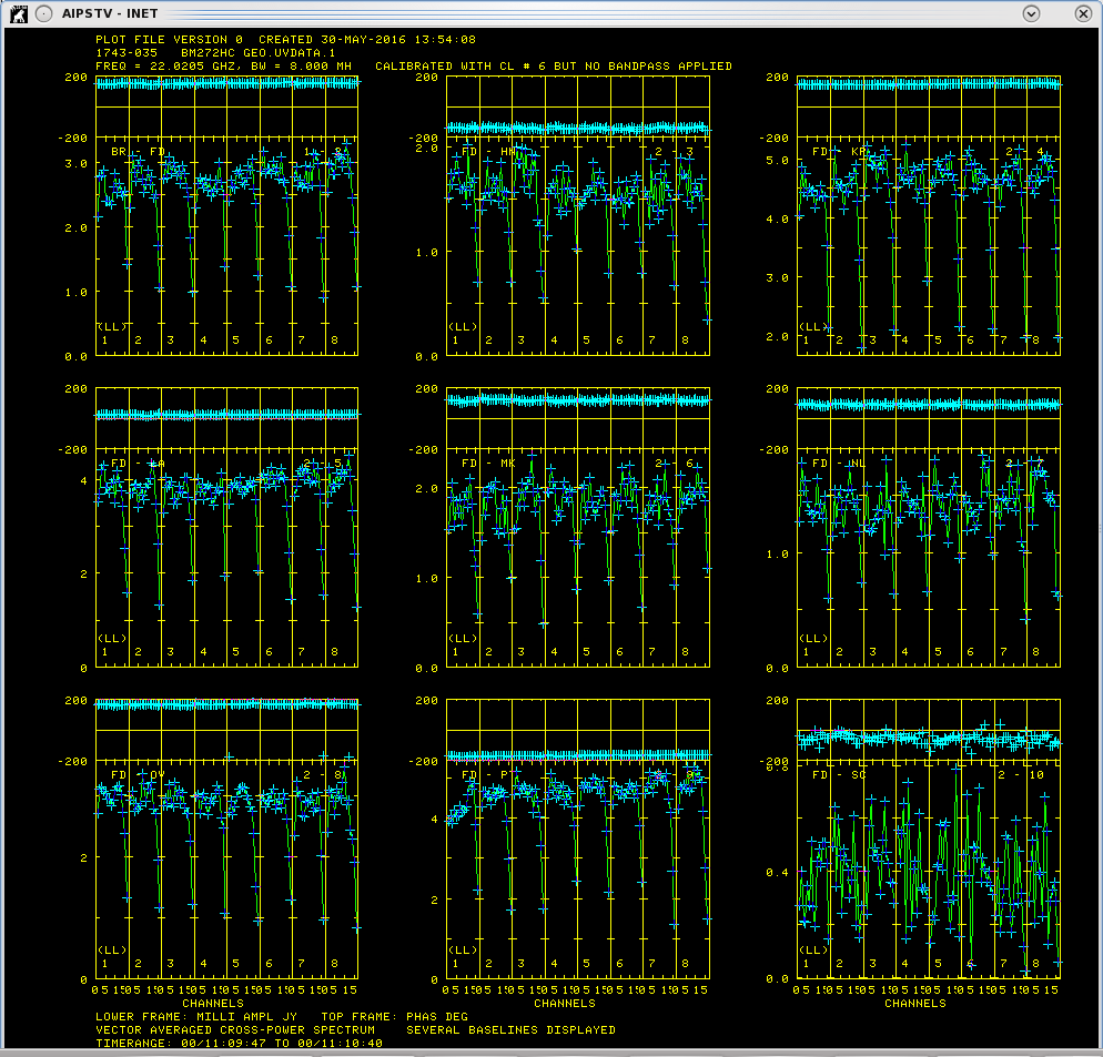
- Now find a scan that has good fringes on all the baselines by running VLBACRPL. VLBACRPL runs POSSM and displays the spectrum of each baseline (to Fort Davis (antenna 2)), with the amplitude on the bottom and the phases on the top.
default vlbacrpl
getn BM272HC GEO UVDATA file
stokes 'half'
refant 2
gainuse 4
solint -1
dotv 1
source ''
inp
vlbacrpl
Although there are several sources/scans to choose from, I choose 1743-035, which has strong fringes on all baselines
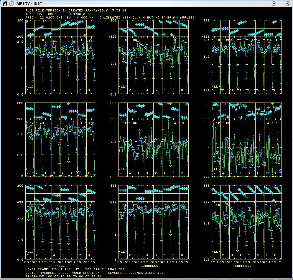 .
.
- Find and remove instrumental delay by running VLBAMPCL.
default vlbampcl
getn BM272HC GEO UVDATA file
calsour '1743-035''
timer 0 7 15 8 0 7 16 01 ➜ scan with good fringes we found in POSSM plots.
refant 2➜ choose reference antenna from in the middle of array, FD (antenna 2) is a good choice.
gainu 4➜ apply highest CL table. Please do an imh here to make sure the highest CL table is really 6.
inp
vlbampcl
At this point you should check on the calibration:
- First check you have no failed solutions. At the end of the FRING run it should tell you how many "good" and "failed" solutions it has found. For this step there must be no failed solutions, failed solutions in this step mean that whatever antenna the failed solution was on is deleted from your data. For this data there should be "80 good solutions".
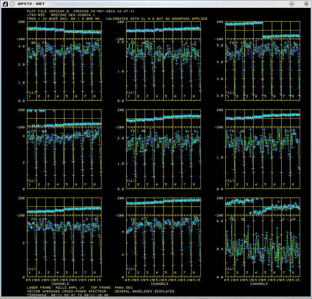
- check solutions in POSSM, the jumps in phase between the IFs should be gone. The phases may also be flattened.
tget possm➜ to "get" all the inputs from the last run (it was run when we ran the procedure VLBACRPL).
gainu 5
inp
go
As you can see that the phase jumps between the IFs are gone, but there is a general phase slope across all the IF, this is the multi-band delay that we will measure and fit for the zenith delay.
- Determine mult-band delay (MBD) by running FRING. This will take a few minutes.
default fring
getn BM272HC GEO UVDATA file
refant 2
doca1 1; gainu 5
aparm(5)=2 ➜ solve form the MBD.
inp
go
There will be alot of failed solutions (~20%) here and that is O.K..
- Check MBD with SNPLT.
default snplt
getn BM272HC GEO UVDATA file
inext 'sn'; invers 3
nplots 10
dotv 1
opty 'mdel'➜ plot MBD.
xaxis 2➜ plot verses elevation.
tvin➜ clear TV.
go
It is important that the MBD be correct because the fitting in DELZN can easily go wonky.
Note that most MBD are between a fraction and a few ns.. Large ones are probably wrong and should be clipped. There also should be a general trend from low to high elecations, although this is not always clear in the plot, the most obvious classic case is for SC in this plot
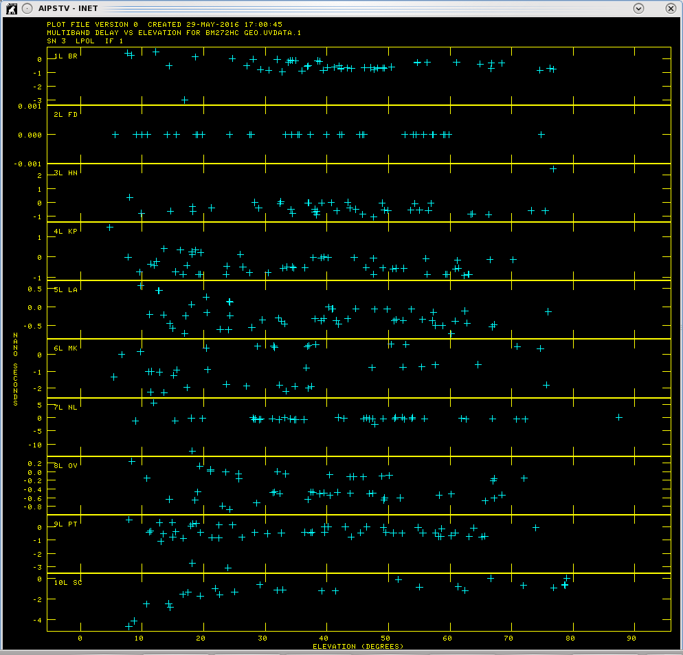 . Make note of the obviously bad points, one at BR (-3 na), one at HN (2 ns) and one at NL (at -10).
- Edit the MBD with SNEDT. SNEDT will only plot vers time, which is why we noted the bad points above.
default snedt
getn BM272HC GEO UVDATA file
inext 'sn'; invers 3
antuse 1 2 3 4 5 6 7 8 9 10
dodelay 2
go
Flag the points noted above.
- Check MBD agian with SNPLT.
tget snplt
invers 4
tvin
go
Looks OK, maybe some more flagging needed, but lets see how DELZN does.
>Solve for zenith and clock delays with DELZN.
default delzn
getn BM272HC GEO UVDATA file
snver 4➜ SN table with edited MBD
gainv 5➜ CL table to copy and correct.
aparm 0 3 2 1 1 10➜ plot zenith atmos. delay; use 3 polynomial terms to fit atmosphere; use 2 polynomial terms to fit clock; create CL table; correct both atmosphere and clock; use 10 iterations of robust fitting.
opty 'mdel'➜ fit MBD.
outfi 'FITS:delzn.clor➜ file to read in with CLCOR; note if you leave of the closing ' the outfi retains the case.
dotv -1➜ don't plot to TV make PL files.
inp
go
DELZN makes plots that I don't find particularly useful to evaluate the quality of the fit. The best way to evaluate this (other than applying it to the astrometric data and see if it improves things) is to apply the CL table that DELZN produces to the GEO data and see if it flattens the MBD across all the IFs. As you can see the results look squite good.
| |
 |
| Before DELZN |
Same scan after DELZN |
Now we transfer these solutions to the target dataset.
This is where it gets a little complicated (although not much). Now we must apply the solutions to the data with the target in it, with
all the calibration except the final fringe fit. The calibrated data
you have has the final fringe fit in it, so we can compare the DELZNed
and non-DELZNed data. So use "imh" on the TARGET (SPLATed) data to see
how many CL tables there are. We want to apply the DELZN solution to the CL table
immediately before the final fringe fit.
- Apply the zenith delay correction with CLCOR.
default clcor
getn BM272HC SPLAT file
opco 'atmo'➜ read in a file of atmospheric and clock delay corrections and apply them to the given CL table.
gainv 1; gainu 0➜ input CL#1; create a new CL table.
infile 'FITS:delzn.clor➜ file with corrections.
inp
go
CLCOR will say it have created CL table #3. Use this for further calibration, i.e. skip CL#2..
Now we repeat steps 18-20 above.
- Do global fring fit with FRING. This is where vput/vget come in handy, if you didn't do the vput, then repeat step 18 but change the gainuse parameter as shown below.
vnum 1; vget fring
gainu 3
inp
go
- Apply calibration to tables with CLCAL. Again either repeat step 19 changing parameters as shown below or use vget.
vnum 1; vget clcal
snver 2
gainv 3
gainu 4
inp
go
- Apply calibration to data with SPLIT. Here we can use tget because SPLIT has not been used since the last time we ran it on this data. Again repeat step 20 if you can't do this.
tget split
gainu 4
outcl 'delzn'
inp
go
- Image J2007+4029 with IMAGR.
tget imagr
cell 3e-5
imsi 512
dotv 1
niter 1000
im2parm 10 6 9 0.5
bchan 0; echan 0
nchav 256
inp
go
Compare this image to the one made without the correction. As you can see the one after the correction has a lower noise level and a source with a higher peak. Bad phases spread the flux around the image and make the noise level higher and source flux lower as well as shifting the position of the source.
| |
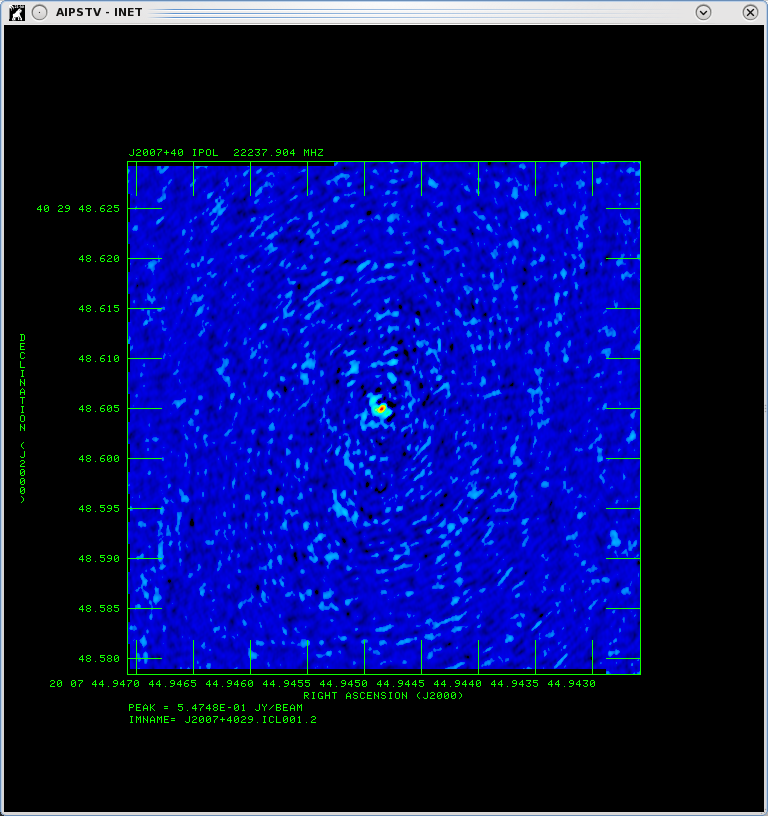 |
| Before DELZN |
After DELZN, plotted with the same pixrange |
If you have any question please contact
Amy Mioduszewski. Last updated 31-May-2016.